Confidence Intervals Confidence Interval We are trying to

Confidence Intervals

Confidence Interval • We are trying to draw a conclusion about a population based on a finite sample • We can not be 100% sure about our conclusion • Instead, we express a confidence interval • The distribution depends upon the statistical variable being considered (e. g. Chi-square distribution for variance)

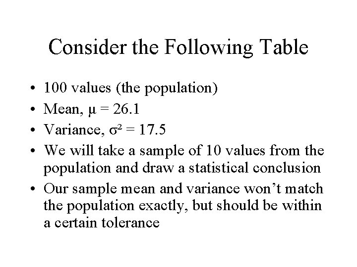
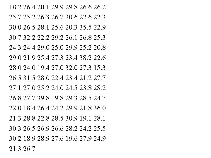
Consider the Following Table • • 100 values (the population) Mean, μ = 26. 1 Variance, σ² = 17. 5 We will take a sample of 10 values from the population and draw a statistical conclusion • Our sample mean and variance won’t match the population exactly, but should be within a certain tolerance

18. 2 26. 4 20. 1 29. 9 29. 8 26. 6 26. 2 25. 7 25. 2 26. 3 26. 7 30. 6 22. 3 30. 0 26. 5 28. 1 25. 6 20. 3 35. 5 22. 9 30. 7 32. 2 29. 2 26. 1 26. 8 25. 3 24. 4 29. 0 25. 0 29. 9 25. 2 20. 8 29. 0 21. 9 25. 4 27. 3 23. 4 38. 2 22. 6 28. 0 24. 0 19. 4 27. 0 32. 0 27. 3 15. 3 26. 5 31. 5 28. 0 22. 4 23. 4 21. 2 27. 7 27. 1 27. 0 25. 2 24. 0 24. 5 23. 8 28. 2 26. 8 27. 7 39. 8 19. 8 29. 3 28. 5 24. 7 22. 0 18. 4 26. 4 24. 2 29. 9 21. 8 36. 0 21. 3 28. 8 22. 8 28. 5 30. 9 19. 1 28. 1 30. 3 26. 5 26. 9 26. 6 28. 2 24. 2 25. 5 30. 2 18. 9 27. 6 19. 6 27. 9 24. 9 21. 3 26. 7

Class Experiment • Randomly select data sets of 10 values • Compute mean and variance for the sample. • Compare to population mean and variance

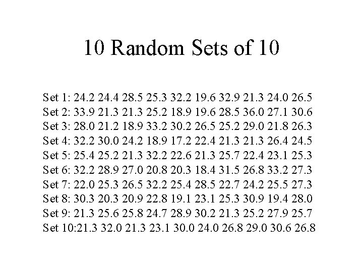
10 Random Sets of 10 Set 1: 24. 2 24. 4 28. 5 25. 3 32. 2 19. 6 32. 9 21. 3 24. 0 26. 5 Set 2: 33. 9 21. 3 25. 2 18. 9 19. 6 28. 5 36. 0 27. 1 30. 6 Set 3: 28. 0 21. 2 18. 9 33. 2 30. 2 26. 5 25. 2 29. 0 21. 8 26. 3 Set 4: 32. 2 30. 0 24. 2 18. 9 17. 2 22. 4 21. 3 26. 4 24. 5 Set 5: 25. 4 25. 2 21. 3 32. 2 22. 6 21. 3 25. 7 22. 4 23. 1 25. 3 Set 6: 32. 2 28. 9 27. 0 20. 8 20. 3 18. 4 31. 5 26. 8 33. 2 27. 3 Set 7: 22. 0 25. 3 26. 5 32. 2 25. 4 28. 5 22. 7 24. 2 25. 5 27. 3 Set 8: 30. 3 20. 9 22. 8 19. 1 23. 1 25. 3 30. 9 19. 4 28. 0 Set 9: 21. 3 25. 6 25. 8 24. 7 28. 9 30. 2 21. 3 25. 2 27. 9 25. 7 Set 10: 21. 3 32. 0 21. 3 23. 1 30. 0 24. 0 26. 8 29. 0 30. 6 26. 8

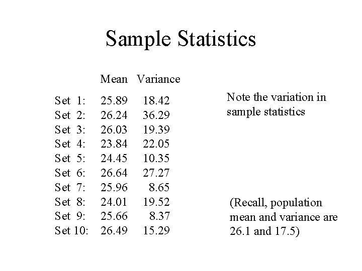
Sample Statistics Mean Variance Set 1: Set 2: Set 3: Set 4: Set 5: Set 6: Set 7: Set 8: Set 9: Set 10: 25. 89 26. 24 26. 03 23. 84 24. 45 26. 64 25. 96 24. 01 25. 66 26. 49 18. 42 36. 29 19. 39 22. 05 10. 35 27. 27 8. 65 19. 52 8. 37 15. 29 Note the variation in sample statistics (Recall, population mean and variance are 26. 1 and 17. 5)

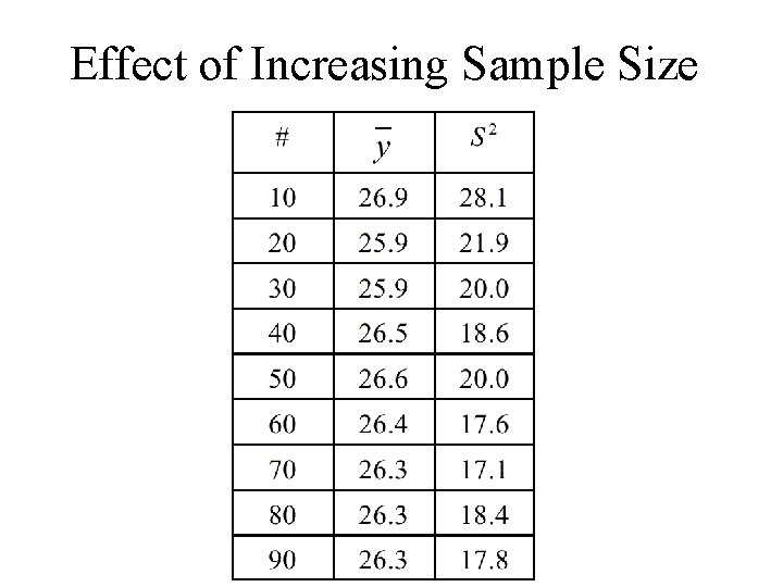
Effect of Increasing Sample Size

Sampling Distribution Theory • Greater confidence with larger samples • We use estimators to make inferences about populations • Two estimators were already discussed – sample mean and sample variance • The estimators themselves are random variables, each having a particular distribution

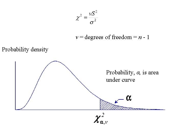
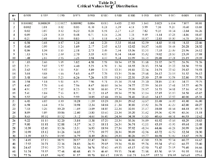
Chi-Square 2 (χ ) Distribution • Compares the relationship between population variance and sample variance • Depends on the sample size and therefore the number of degrees of freedom • Not symmetric – skewed to the right

v = degrees of freedom = n - 1 Probability density Probability, α, is area under curve

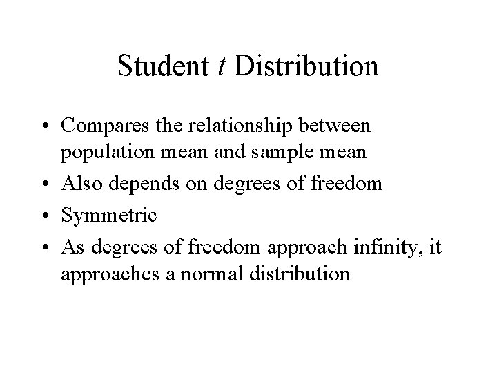
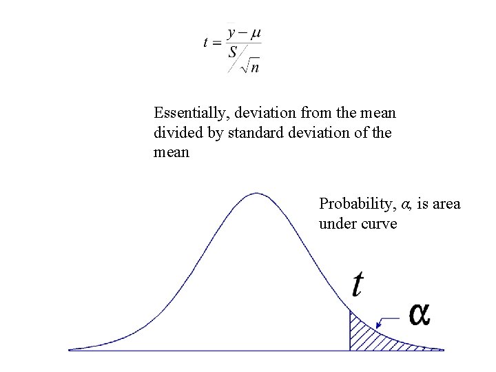
Student t Distribution • Compares the relationship between population mean and sample mean • Also depends on degrees of freedom • Symmetric • As degrees of freedom approach infinity, it approaches a normal distribution

Essentially, deviation from the mean divided by standard deviation of the mean Probability, α, is area under curve

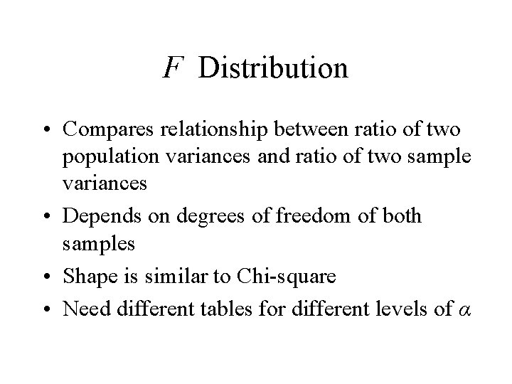
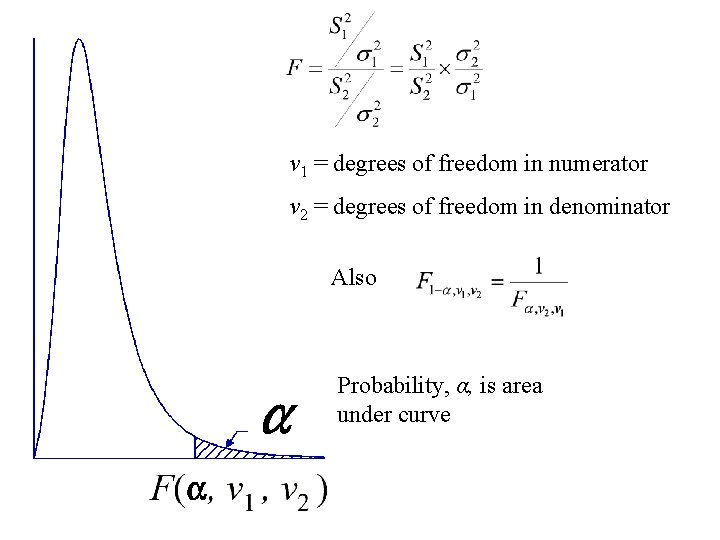
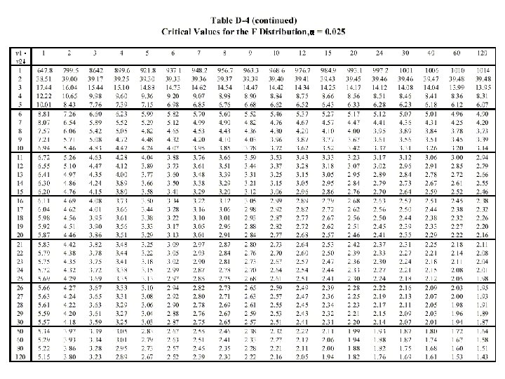
F Distribution • Compares relationship between ratio of two population variances and ratio of two sample variances • Depends on degrees of freedom of both samples • Shape is similar to Chi-square • Need different tables for different levels of α

v 1 = degrees of freedom in numerator v 2 = degrees of freedom in denominator Also Probability, α, is area under curve

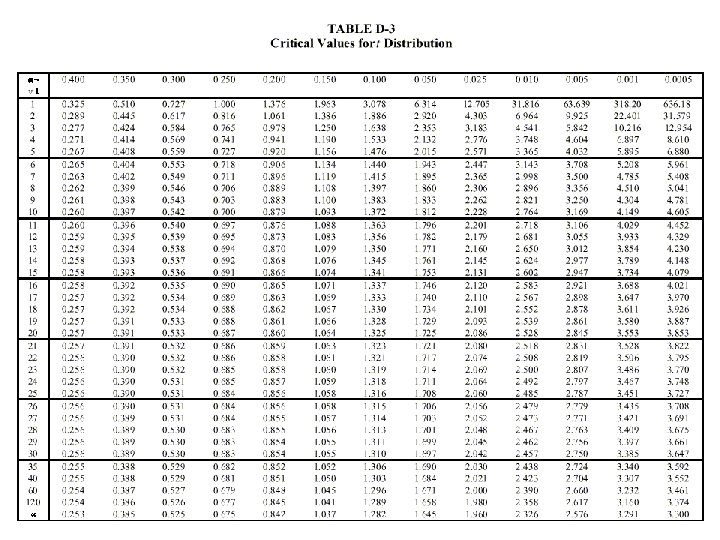
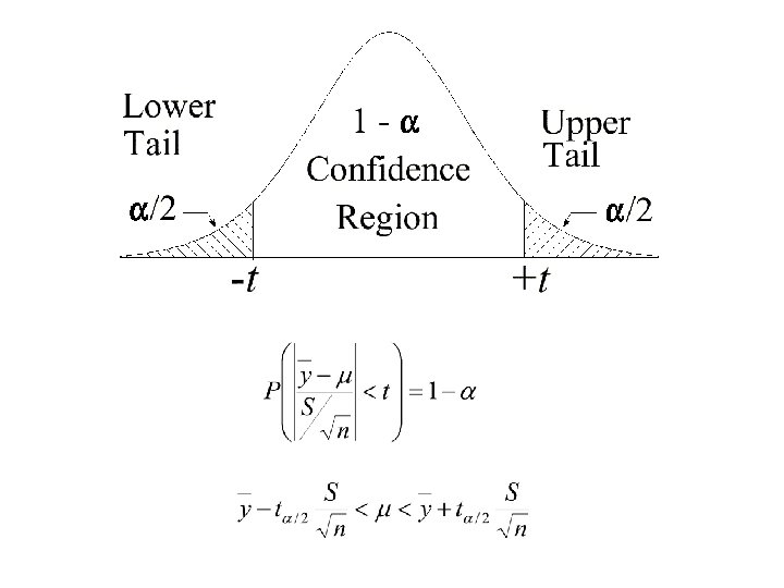
Confidence Interval for the Mean • Normal distribution is used for populations • For finite samples, use the Student-t distribution • Once the sample size reaches about 30, the distribution becomes approximately normal (to about 2 significant figures) • For an interval, divide probability, α, by 2 for correct t-table value

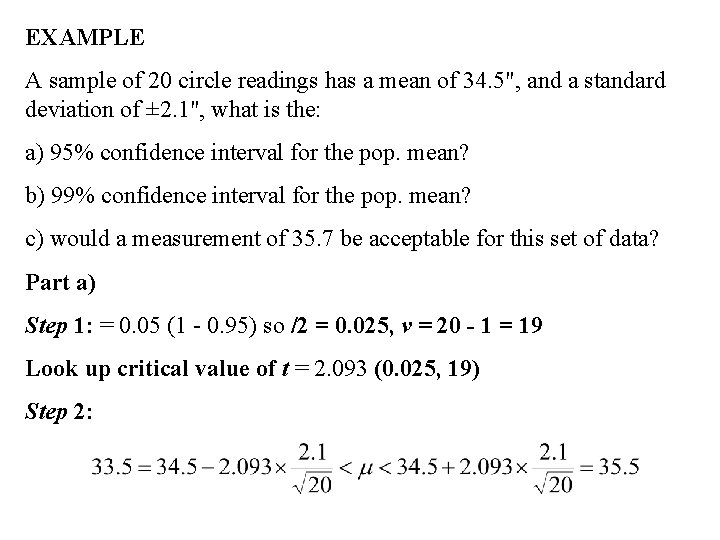
EXAMPLE A sample of 20 circle readings has a mean of 34. 5", and a standard deviation of ± 2. 1", what is the: a) 95% confidence interval for the pop. mean? b) 99% confidence interval for the pop. mean? c) would a measurement of 35. 7 be acceptable for this set of data? Part a) Step 1: = 0. 05 (1 - 0. 95) so /2 = 0. 025, v = 20 - 1 = 19 Look up critical value of t = 2. 093 (0. 025, 19) Step 2:

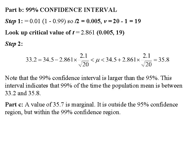
Part b: 99% CONFIDENCE INTERVAL Step 1: = 0. 01 (1 - 0. 99) so /2 = 0. 005, v = 20 - 1 = 19 Look up critical value of t = 2. 861 (0. 005, 19) Step 2: Note that the 99% confidence interval is larger than the 95%. This interval indicates that 99% of the time the population mean is between 33. 2 and 35. 8. Part c: A value of 35. 7 is marginal. It is outside the 95% confidence region, but within the 99% confidence region.

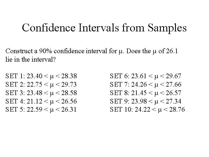
Confidence Intervals from Samples Construct a 90% confidence interval for µ. Does the µ of 26. 1 lie in the interval? SET 1: 23. 40 < µ < 28. 38 SET 2: 22. 75 < µ < 29. 73 SET 3: 23. 48 < µ < 28. 58 SET 4: 21. 12 < µ < 26. 56 SET 5: 22. 59 < µ < 26. 31 SET 6: 23. 61 < µ < 29. 67 SET 7: 24. 26 < µ < 27. 66 SET 8: 21. 45 < µ < 26. 57 SET 9: 23. 98 < µ < 27. 34 SET 10: 24. 22 < µ < 28. 76

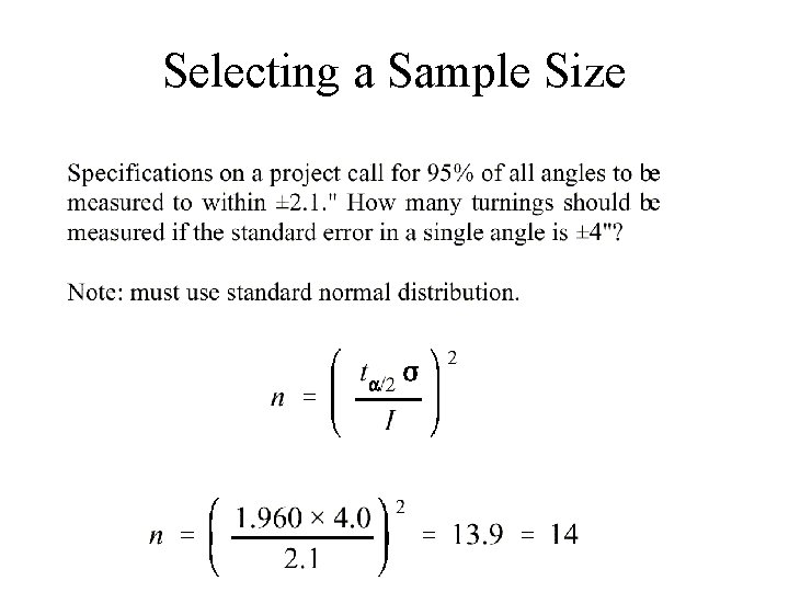
Selecting a Sample Size

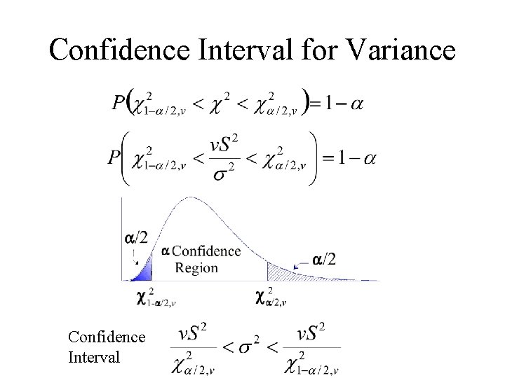
Confidence Interval for Variance Confidence Interval

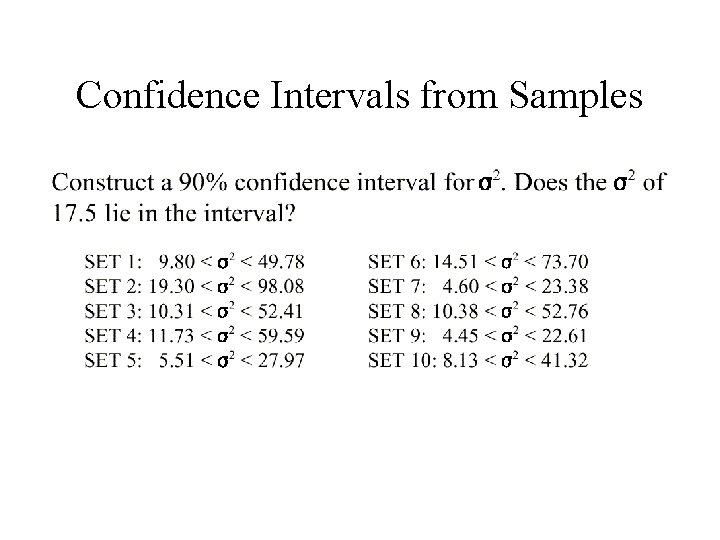
Confidence Intervals from Samples

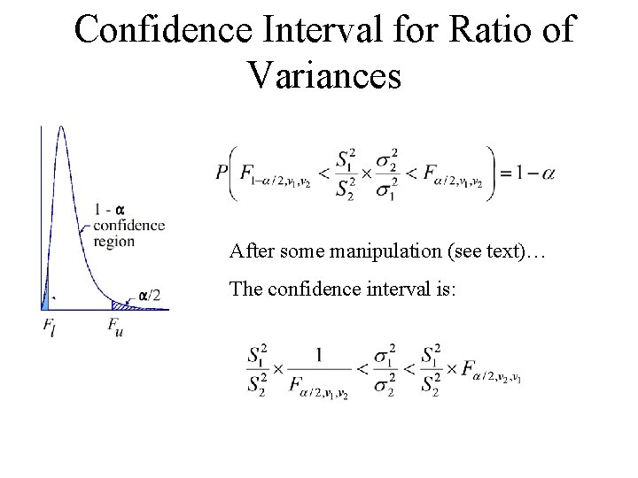
Confidence Interval for Ratio of Variances After some manipulation (see text)… The confidence interval is:

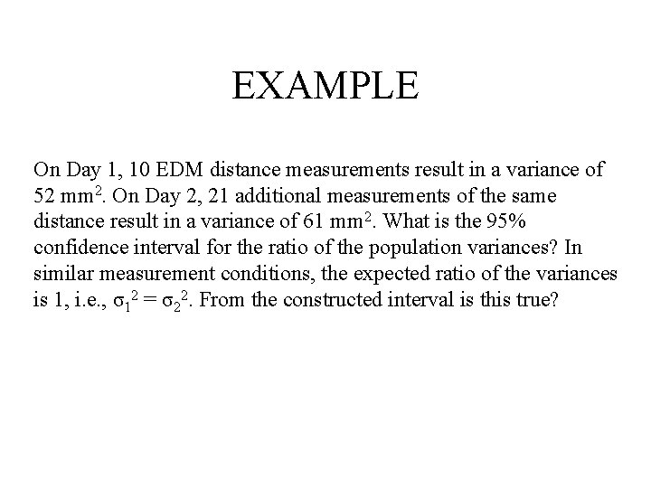
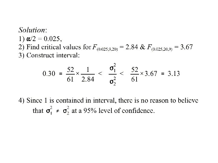
EXAMPLE On Day 1, 10 EDM distance measurements result in a variance of 52 mm 2. On Day 2, 21 additional measurements of the same distance result in a variance of 61 mm 2. What is the 95% confidence interval for the ratio of the population variances? In similar measurement conditions, the expected ratio of the variances is 1, i. e. , σ12 = σ22. From the constructed interval is this true?

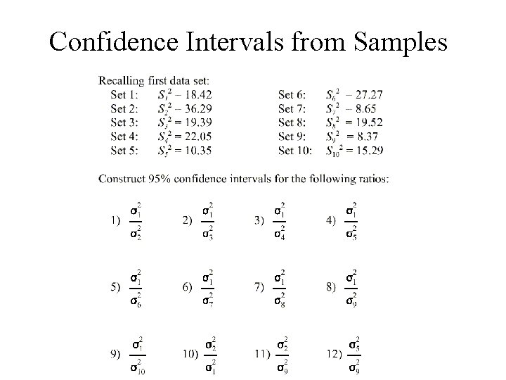
Confidence Intervals from Samples

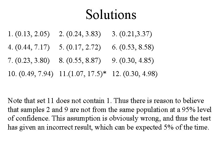
Solutions 1. (0. 13, 2. 05) 2. (0. 24, 3. 83) 3. (0. 21, 3. 37) 4. (0. 44, 7. 17) 5. (0. 17, 2. 72) 6. (0. 53, 8. 58) 7. (0. 23, 3. 80) 8. (0. 55, 8. 87) 9. (0. 30, 4. 85) 10. (0. 49, 7. 94) 11. (1. 07, 17. 5)* 12. (0. 30, 4. 98) Note that set 11 does not contain 1. Thus there is reason to believe that samples 2 and 9 are not from the same population at a 95% level of confidence. This assumption is obviously wrong, and thus the test has given an incorrect result, which can be expected 5% of the time.