Lecture 14 Thurs Oct 23 Multiple Comparisons Sections

Lecture 14 – Thurs, Oct 23 • Multiple Comparisons (Sections 6. 3, 6. 4). • Next time: Simple linear regression (Sections 7. 1 -7. 3)

Compound Uncertainty • Compound uncertainty: When drawing more than one direct inference, there is an increased chance of making at least one mistake. • Impact on tests: If using a conventional criteria such as a p-value of 0. 05 to reject a null hypothesis, the probability of falsely rejecting a null hypothesis will be greater than 0. 05 if considering multiple tests. • Impact on confidence intervals: If forming multiple 95% confidence intervals, the chance that all of the confidence intervals will contain true parameter is less than 95%.

Simultaneous Inferences • When several 95% confidence intervals are considered simultaneously, they constitute a family of confidence intervals • Individual Confidence Level: Success rate of a procedure for constructing a single confidence interval. • Familywise Confidence Level: Success rate of procedure for constructing a family of confidence intervals, where a “successful” usage is one in which all intervals in the family capture their parameters.

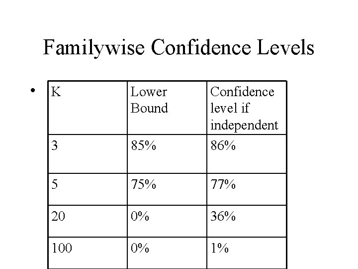
Individual vs. Family Confidence Levels • If a family consists of k confidence intervals, each with individual confidence level 95%, the familywise confidence levels can be no larger than 95% and no smaller than 100(1 -. 05 k)%. • Actual familywise confidence levels depends on degree of dependence between intervals. • If the intervals are independent, the familywise confidence level is 100(. 95)k%.

Familywise Confidence Levels • K Lower Bound 3 85% Confidence level if independent 86% 5 75% 77% 20 0% 36% 100 0% 1%

Multiple Comparison Procedures • Multiple comparison procedures are methods of constructing individual confidence intervals so that familywise confidence level is controlled (at 95% for example). • Key issue: What is the appropriate family to consider?

Planned vs. Unplanned Comparisons • Consider one-way classification with 20 groups. • Planned Comparisons: researcher is specifically interested in comparing groups 1 and 4 because comparison answers a research question directly. This is a planned comparison. In the mice diets example, the researchers had five planned comparisons. • Unplanned Comparisons: researcher examines all possible pairs of groups – 190 groups. As a result, researcher finds that only groups 5 and 8 suggest actual differences. Only this pair is reported as significant.

Families in Planned/Unplanned • Planned Comparisons: The family of confidence intervals is the family of all planned comparison confidence intervals (e. g. , the family of five planned comparisons in mice diet). For small number of planned comparisons, it is usual practice to just use individual confidence intervals controlled at 95%. • Unplanned Comparisons: The family of confidence intervals is the family of all possible comparisons - (k*(k-1)/2) for a k-group one-way classification. It is important to control the familywise confidence level for unplanned comps.

Multiple Comparison Procedures • Confidence Interval: Estimate Margin of Error = (Multiplier)x(Standard Error of Estimate). For multiple comparison procedures, the multipliers is greater than the usual 2. • Multiple comparisons procedures – Tukey/Kramer’s “Honest Significant Differences” – Bonferroni

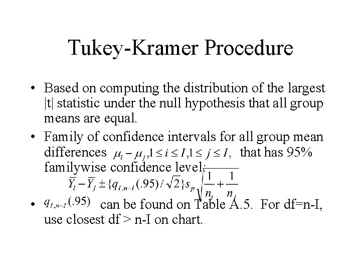
Tukey-Kramer Procedure • Based on computing the distribution of the largest |t| statistic under the null hypothesis that all group means are equal. • Family of confidence intervals for all group mean differences that has 95% familywise confidence level: • can be found on Table A. 5. For df=n-I, use closest df > n-I on chart.

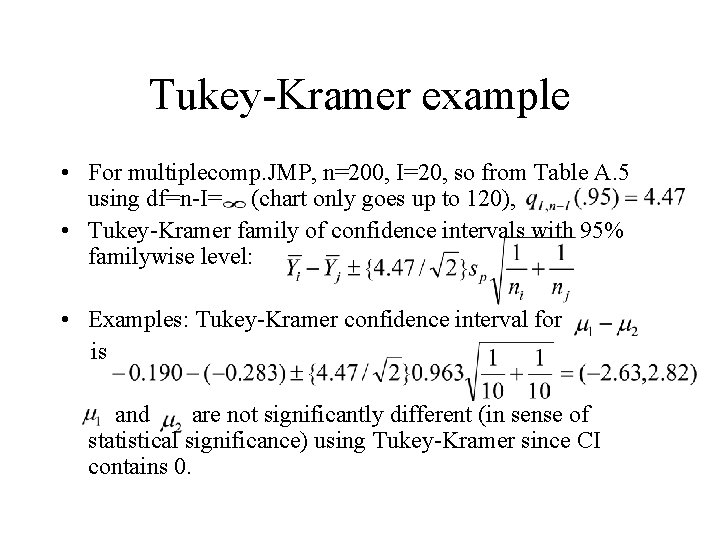
Tukey-Kramer example • For multiplecomp. JMP, n=200, I=20, so from Table A. 5 using df=n-I= (chart only goes up to 120), • Tukey-Kramer family of confidence intervals with 95% familywise level: • Examples: Tukey-Kramer confidence interval for is and are not significantly different (in sense of statistical significance) using Tukey-Kramer since CI contains 0.

Tukey-Kramer in JMP • To see which groups are significantly different (in sense of statistical significance), i. e. , which groups have CI for difference in group means that does not contain 0, click Compare Means under Oneway Analysis (after Analyze, Fit Y by X) and click All Pairs, Tukey’s HSD. • In table “Comparison of All Pairs Using Tukey’s HSD, ” two groups are significantly different if and only if the entry in the table for the pair of groups is positive.

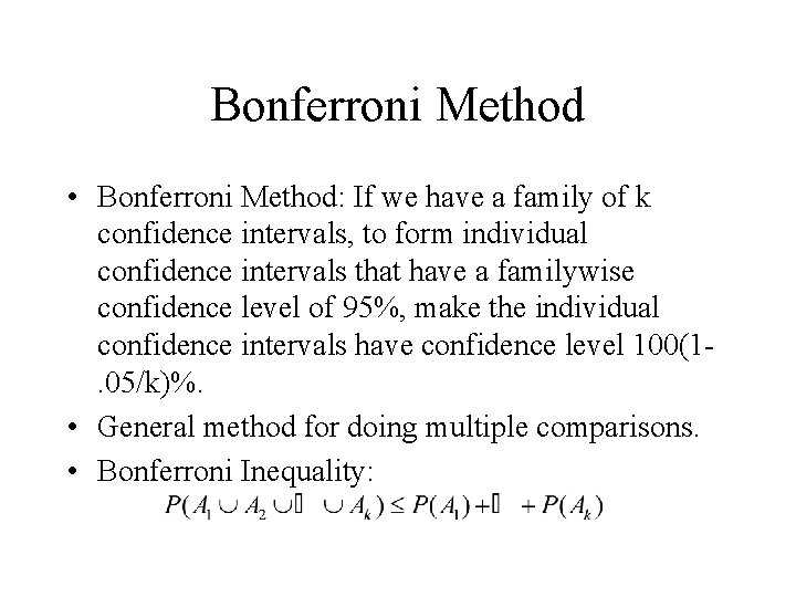
Bonferroni Method • Bonferroni Method: If we have a family of k confidence intervals, to form individual confidence intervals that have a familywise confidence level of 95%, make the individual confidence intervals have confidence level 100(1. 05/k)%. • General method for doing multiple comparisons. • Bonferroni Inequality:

Bonferroni for tests • Suppose we are conducting k hypothesis tests and will “reject” the null hypothesis if the p-value is smaller than a cutoff p* (e. g. , p* =. 05). • Per-test type I error rate: the probability of falsely rejecting the null hypothesis when it is true. The per-test type I error rate is p*. • Familywise error rate: the probability of falsely rejecting at least one null hypothesis in a family of tests when all null hypotheses are true. • Bonferroni for tests: For a family of k tests, use a cutoff of p*/k to obtain a familywise error rate of at most p*, e. g. , for ten tests, reject if p-value <0. 005 to obtain familywise error rate of at most 0. 05.

Bonferroni for mice diets • Five comparisons were planned. Suppose we want the familywise error rate for the five comparisons to be 0. 05. • Bonferroni method: We should consider two groups to be significantly different if the pvalue from the two-sided t-test is less than 0. 05/5=0. 01. •

Exploratory Data Analysis and Multiple Comparisons • Searching data for suggestive patterns can lead to important discoveries but it is difficult to test a hypothesis against a data set which suggested it. We must protect against “data snooping. ” • One way to try to protect against data snooping is to use multiple comparisons procedures (e. g. , example in Section 6. 5. 2). • The best way to protect against data snooping is to design a study to search specifically for a pattern that was suggested by an exploratory data analysis. In other words we convert an “unplanned” comparison into a “planned” comparison by doing a new experiment.

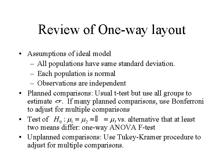
Review of One-way layout • Assumptions of ideal model – All populations have same standard deviation. – Each population is normal – Observations are independent • Planned comparisons: Usual t-test but use all groups to estimate. If many planned comparisons, use Bonferroni to adjust for multiple comparisons • Test of vs. alternative that at least two means differ: one-way ANOVA F-test • Unplanned comparisons: Use Tukey-Kramer procedure to adjust for multiple comparisons.

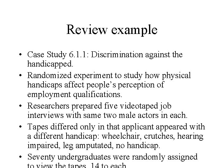
Review example • Case Study 6. 1. 1: Discrimination against the handicapped. • Randomized experiment to study how physical handicaps affect people’s perception of employment qualifications. • Researchers prepared five videotaped job interviews with same two male actors in each. • Tapes differed only in that applicant appeared with a different handicap: wheelchair, crutches, hearing impaired, leg amputated, no handicap. • Seventy undergraduates were randomly assigned