CMSC 723 LING 645 Intro to Computational Linguistics

CMSC 723 / LING 645: Intro to Computational Linguistics February 25, 2004 Lecture 5 (Dorr): Intro to Probabilistic NLP and N-grams (chap 6. 1 -6. 3) Prof. Bonnie J. Dorr Dr. Nizar Habash TA: Nitin Madnani, Nate Waisbrot

Why (not) Statistics for NLP? ¬Pro – Disambiguation – Error Tolerant – Learnable ¬Con – Not always appropriate – Difficult to debug

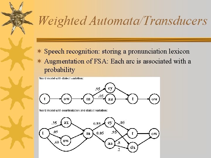
Weighted Automata/Transducers ¬ Speech recognition: storing a pronunciation lexicon ¬ Augmentation of FSA: Each arc is associated with a probability

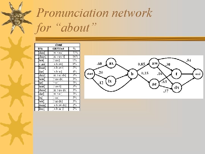
Pronunciation network for “about”

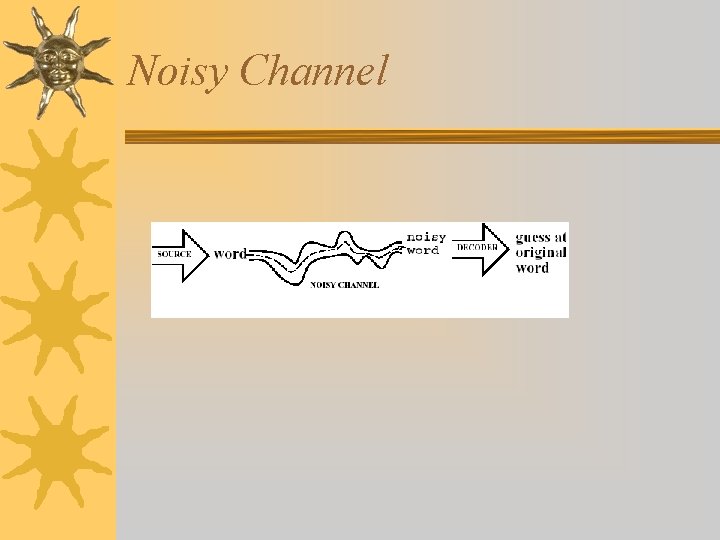
Noisy Channel

Probability Definitions ¬ Experiment (trial) – Repeatable procedure with well-defined possible outcomes ¬ Sample space – Complete set of outcomes ¬ Event – Any subset of outcomes from sample space ¬ Random Variable – Uncertain outcome in a trial

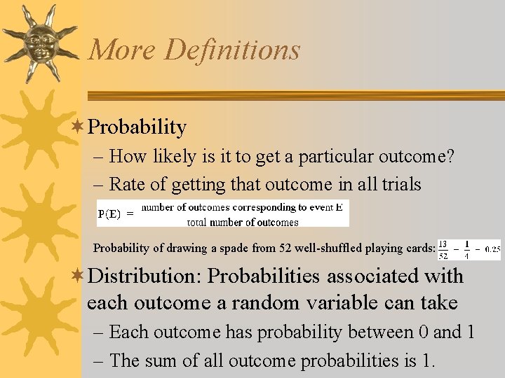
More Definitions ¬Probability – How likely is it to get a particular outcome? – Rate of getting that outcome in all trials Probability of drawing a spade from 52 well-shuffled playing cards: ¬Distribution: Probabilities associated with each outcome a random variable can take – Each outcome has probability between 0 and 1 – The sum of all outcome probabilities is 1.

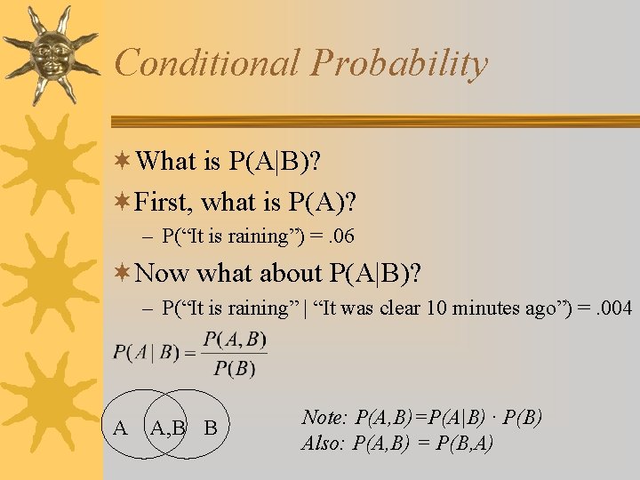
Conditional Probability ¬What is P(A|B)? ¬First, what is P(A)? – P(“It is raining”) =. 06 ¬Now what about P(A|B)? – P(“It is raining” | “It was clear 10 minutes ago”) =. 004 A A, B B Note: P(A, B)=P(A|B) · P(B) Also: P(A, B) = P(B, A)

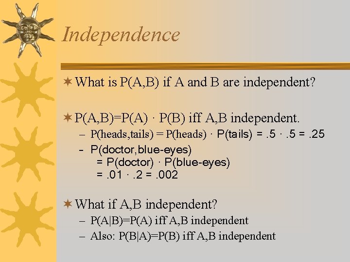
Independence ¬ What is P(A, B) if A and B are independent? ¬ P(A, B)=P(A) · P(B) iff A, B independent. – P(heads, tails) = P(heads) · P(tails) =. 5 ·. 5 =. 25 – P(doctor, blue-eyes) = P(doctor) · P(blue-eyes) =. 01 ·. 2 =. 002 ¬ What if A, B independent? – P(A|B)=P(A) iff A, B independent – Also: P(B|A)=P(B) iff A, B independent

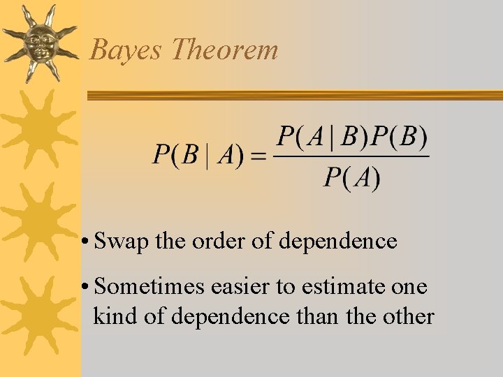
Bayes Theorem • Swap the order of dependence • Sometimes easier to estimate one kind of dependence than the other

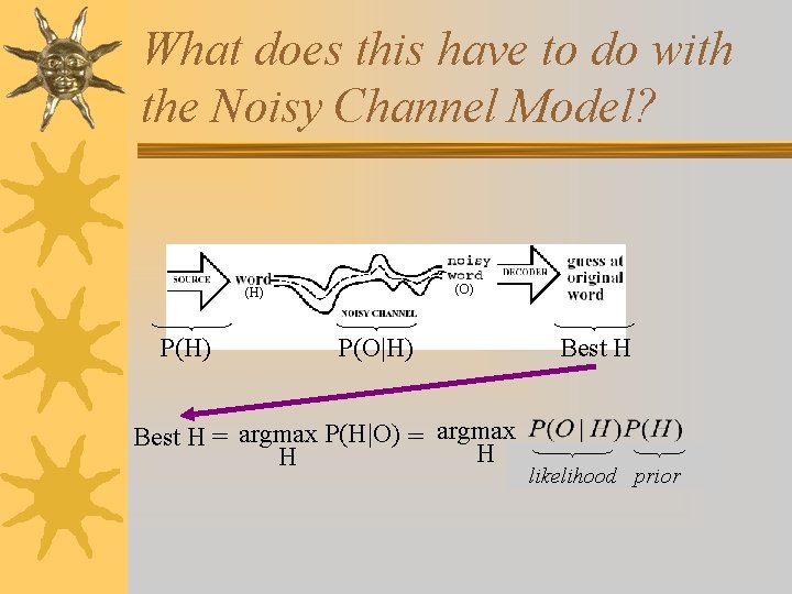
What does this have to do with the Noisy Channel Model? (O) (H) P(O|H) Best H = argmax P(H|O) = argmax H H Best H likelihood prior

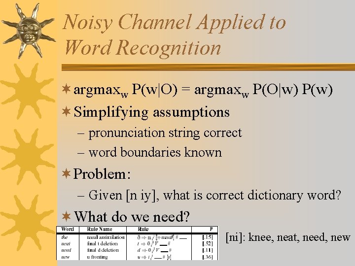
Noisy Channel Applied to Word Recognition ¬argmaxw P(w|O) = argmaxw P(O|w) P(w) ¬Simplifying assumptions – pronunciation string correct – word boundaries known ¬Problem: – Given [n iy], what is correct dictionary word? ¬What do we need? [ni]: knee, neat, need, new

What is the most likely word given [ni]? ¬ Compute prior P(w) Word freq(w) P(w) new 2625 . 001 neat 338 . 00013 need 1417 . 00056 knee 61 . 000024 ¬ Now compute likelihood P([ni]|w), then multiply Word P(O|w)P(w) new . 36 . 001 . 00036 neat . 52 . 00013 . 000068 need . 11 . 00056 . 000062 knee 1. 000024

Why N-grams? ¬ Compute likelihood P([ni]|w), then multiply Word P(O|w)P(w) new . 36 . 001 . 00036 P([ni]|new)P(new) neat . 52 . 00013 . 000068 P([ni]|neat)P(neat) need . 11 . 00056 . 000062 P([ni]|need)P(need) knee 1. 000024 P([ni]|knee)P(knee) ¬Unigram approach: ignores context ¬Need to factor in context (n-gram) - Use P(need|I) instead of just P(need) - Note: P(new|I) < P(need|I)

Next Word Prediction [borrowed from J. Hirschberg] From a NY Times story. . . – Stocks plunged this …. – Stocks plunged this morning, despite a cut in interest rates by the Federal Reserve, as Wall. . . – Stocks plunged this morning, despite a cut in interest rates by the Federal Reserve, as Wall Street began

Next Word Prediction (cont) – Stocks plunged this morning, despite a cut in interest rates by the Federal Reserve, as Wall Street began trading for the first time since last … – Stocks plunged this morning, despite a cut in interest rates by the Federal Reserve, as Wall Street began trading for the first time since last Tuesday's terrorist attacks.

Human Word Prediction ¬Domain knowledge ¬Syntactic knowledge ¬Lexical knowledge

Claim ¬A useful part of the knowledge needed to allow Word Prediction can be captured using simple statistical techniques. ¬Compute: – probability of a sequence – likelihood of words co-occurring

Why would we want to do this? ¬Rank the likelihood of sequences containing various alternative hypotheses ¬Assess the likelihood of a hypothesis

Why is this useful? ¬Speech recognition ¬Handwriting recognition ¬Spelling correction ¬Machine translation systems ¬Optical character recognizers

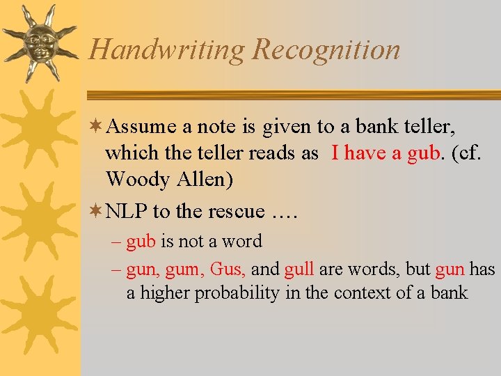
Handwriting Recognition ¬Assume a note is given to a bank teller, which the teller reads as I have a gub. (cf. Woody Allen) ¬NLP to the rescue …. – gub is not a word – gun, gum, Gus, and gull are words, but gun has a higher probability in the context of a bank

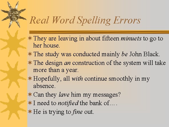
Real Word Spelling Errors ¬ They are leaving in about fifteen minuets to go to her house. ¬ The study was conducted mainly be John Black. ¬ The design an construction of the system will take more than a year. ¬ Hopefully, all with continue smoothly in my absence. ¬ Can they lave him my messages? ¬ I need to notified the bank of…. ¬ He is trying to fine out.

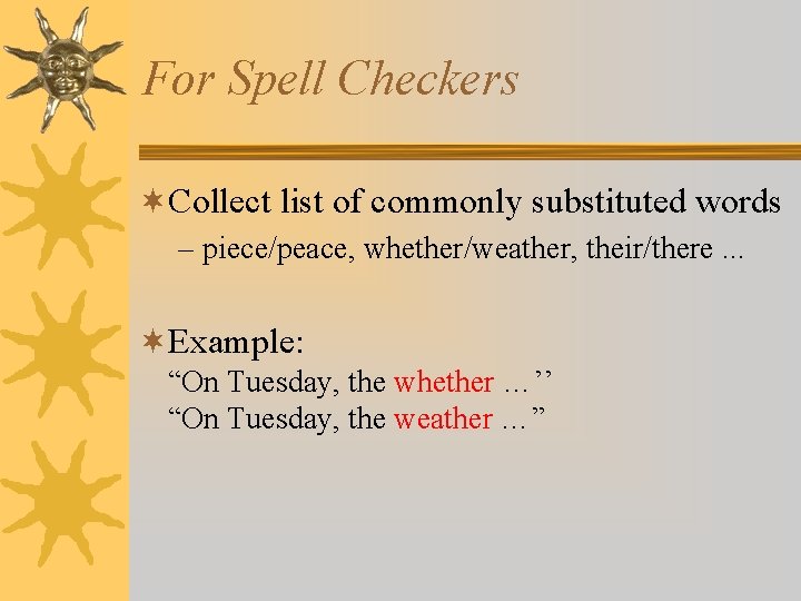
For Spell Checkers ¬Collect list of commonly substituted words – piece/peace, whether/weather, their/there. . . ¬Example: “On Tuesday, the whether …’’ “On Tuesday, the weather …”

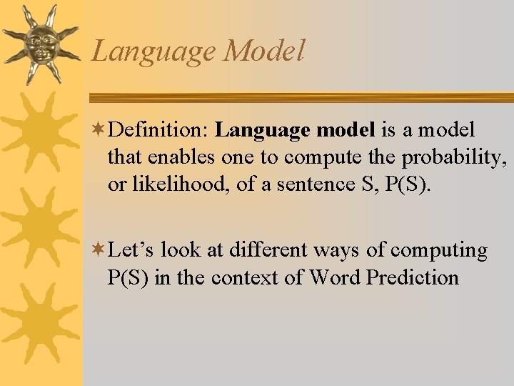
Language Model ¬Definition: Language model is a model that enables one to compute the probability, or likelihood, of a sentence S, P(S). ¬Let’s look at different ways of computing P(S) in the context of Word Prediction

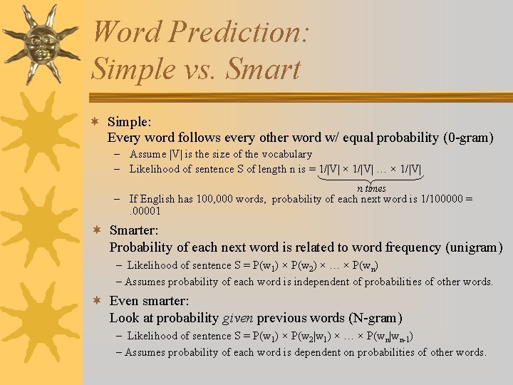
Word Prediction: Simple vs. Smart ¬ Simple: Every word follows every other word w/ equal probability (0 -gram) – Assume |V| is the size of the vocabulary – Likelihood of sentence S of length n is = 1/|V| × 1/|V| … × 1/|V| n times – If English has 100, 000 words, probability of each next word is 1/100000 =. 00001 ¬ Smarter: Probability of each next word is related to word frequency (unigram) – Likelihood of sentence S = P(w 1) × P(w 2) × … × P(wn) – Assumes probability of each word is independent of probabilities of other words. ¬ Even smarter: Look at probability given previous words (N-gram) – Likelihood of sentence S = P(w 1) × P(w 2|w 1) × … × P(wn|wn-1) – Assumes probability of each word is dependent on probabilities of other words.

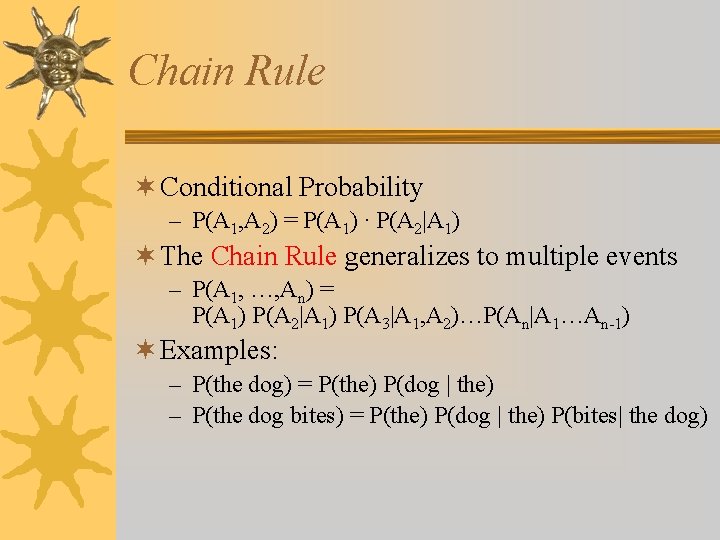
Chain Rule ¬ Conditional Probability – P(A 1, A 2) = P(A 1) · P(A 2|A 1) ¬ The Chain Rule generalizes to multiple events – P(A 1, …, An) = P(A 1) P(A 2|A 1) P(A 3|A 1, A 2)…P(An|A 1…An-1) ¬ Examples: – P(the dog) = P(the) P(dog | the) – P(the dog bites) = P(the) P(dog | the) P(bites| the dog)

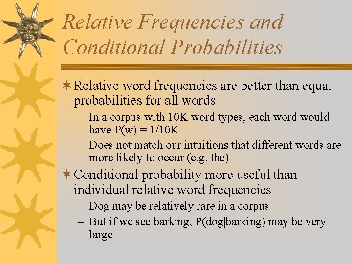
Relative Frequencies and Conditional Probabilities ¬ Relative word frequencies are better than equal probabilities for all words – In a corpus with 10 K word types, each word would have P(w) = 1/10 K – Does not match our intuitions that different words are more likely to occur (e. g. the) ¬ Conditional probability more useful than individual relative word frequencies – Dog may be relatively rare in a corpus – But if we see barking, P(dog|barking) may be very large

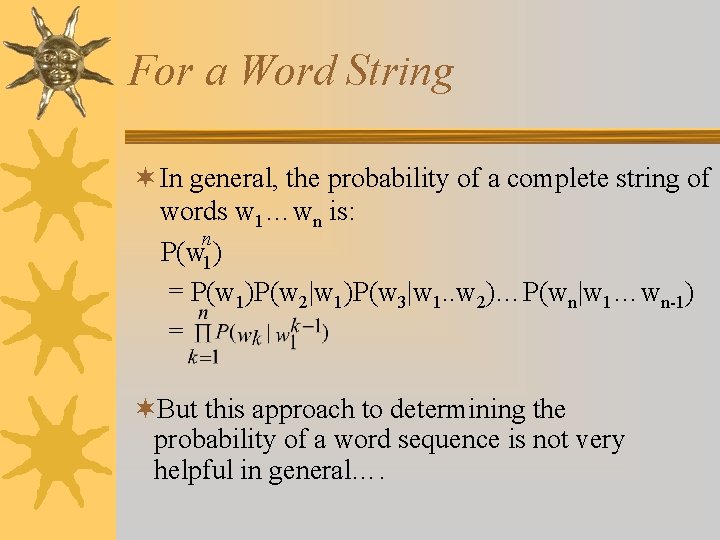
For a Word String ¬ In general, the probability of a complete string of words w 1…wn is: n P(w 1 ) = P(w 1)P(w 2|w 1)P(w 3|w 1. . w 2)…P(wn|w 1…wn-1) = ¬But this approach to determining the probability of a word sequence is not very helpful in general….

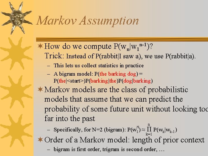
Markov Assumption ¬ How do we compute P(wn|w 1 n-1)? Trick: Instead of P(rabbit|I saw a), we use P(rabbit|a). – This lets us collect statistics in practice – A bigram model: P(the barking dog) = P(the|<start>)P(barking|the)P(dog|barking) ¬ Markov models are the class of probabilistic models that assume that we can predict the probability of some future unit without looking too far into the past n n – Specifically, for N=2 (bigram): P(w 1) ≈ Π P(wk|wk-1) k=1 ¬ Order of a Markov model: length of prior context – bigram is first order, trigram is second order, …

Counting Words in Corpora ¬What is a word? – e. g. , are cat and cats the same word? – September and Sept? – zero and oh? – Is seventy-two one word or two? AT&T? – Punctuation? ¬How many words are there in English? ¬Where do we find the things to count?

Corpora ¬ Corpora are (generally online) collections of text and speech ¬ Examples: – – – Brown Corpus (1 M words) Wall Street Journal and AP News corpora ATIS, Broadcast News (speech) TDT (text and speech) Switchboard, Call Home (speech) TRAINS, FM Radio (speech)

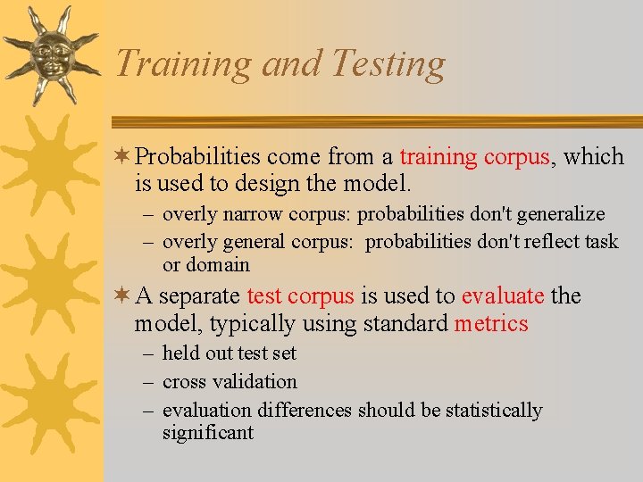
Training and Testing ¬ Probabilities come from a training corpus, which is used to design the model. – overly narrow corpus: probabilities don't generalize – overly general corpus: probabilities don't reflect task or domain ¬ A separate test corpus is used to evaluate the model, typically using standard metrics – held out test set – cross validation – evaluation differences should be statistically significant

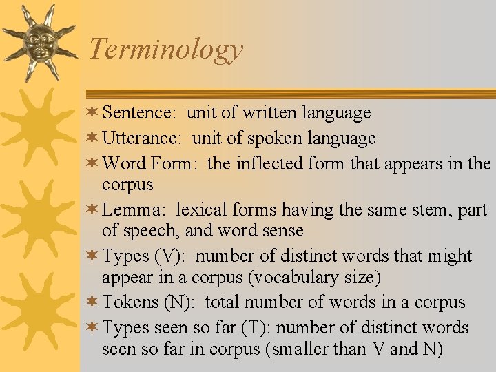
Terminology ¬ Sentence: unit of written language ¬ Utterance: unit of spoken language ¬ Word Form: the inflected form that appears in the corpus ¬ Lemma: lexical forms having the same stem, part of speech, and word sense ¬ Types (V): number of distinct words that might appear in a corpus (vocabulary size) ¬ Tokens (N): total number of words in a corpus ¬ Types seen so far (T): number of distinct words seen so far in corpus (smaller than V and N)

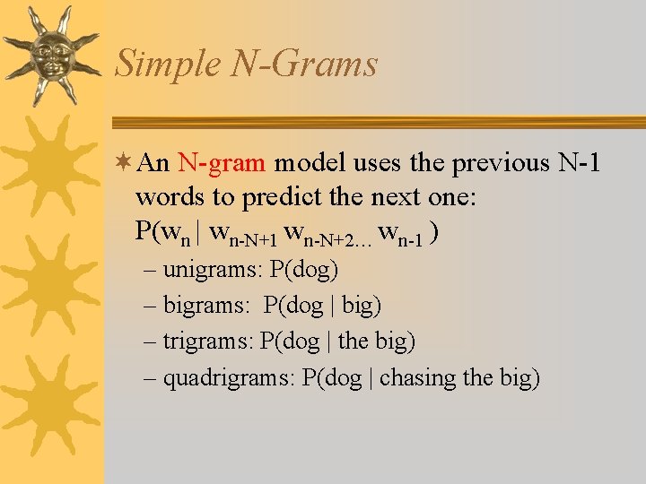
Simple N-Grams ¬An N-gram model uses the previous N-1 words to predict the next one: P(wn | wn-N+1 wn-N+2… wn-1 ) – unigrams: P(dog) – bigrams: P(dog | big) – trigrams: P(dog | the big) – quadrigrams: P(dog | chasing the big)

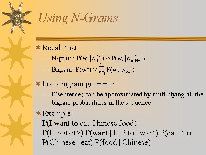
Using N-Grams ¬ Recall that – N-gram: P(wn|w 1 n-1) ≈ P(wn|wn-1 n-N+1) – Bigram: P(wn 1) n ≈Π P(wk|wk-1) k=1 ¬ For a bigrammar – P(sentence) can be approximated by multiplying all the bigram probabilities in the sequence ¬ Example: P(I want to eat Chinese food) = P(I | <start>) P(want | I) P(to | want) P(eat | to) P(Chinese | eat) P(food | Chinese)

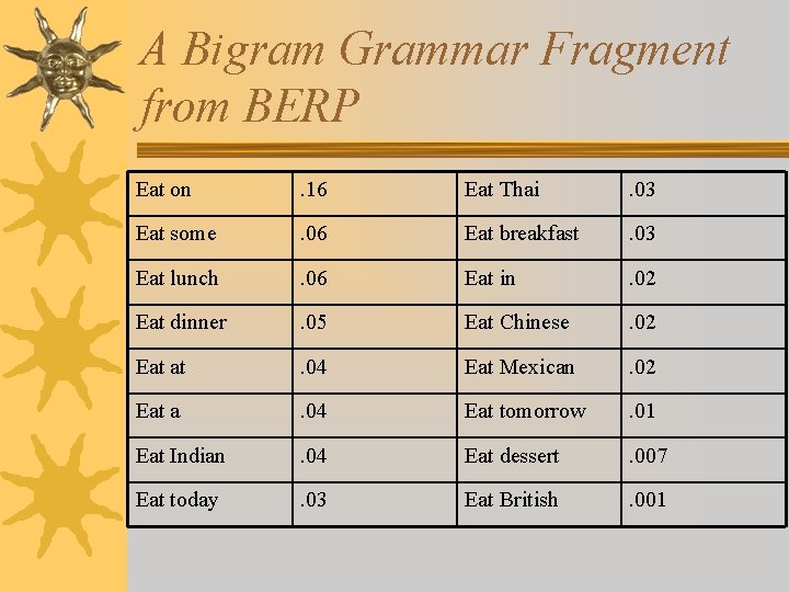
A Bigram Grammar Fragment from BERP Eat on . 16 Eat Thai . 03 Eat some . 06 Eat breakfast . 03 Eat lunch . 06 Eat in . 02 Eat dinner . 05 Eat Chinese . 02 Eat at . 04 Eat Mexican . 02 Eat a . 04 Eat tomorrow . 01 Eat Indian . 04 Eat dessert . 007 Eat today . 03 Eat British . 001

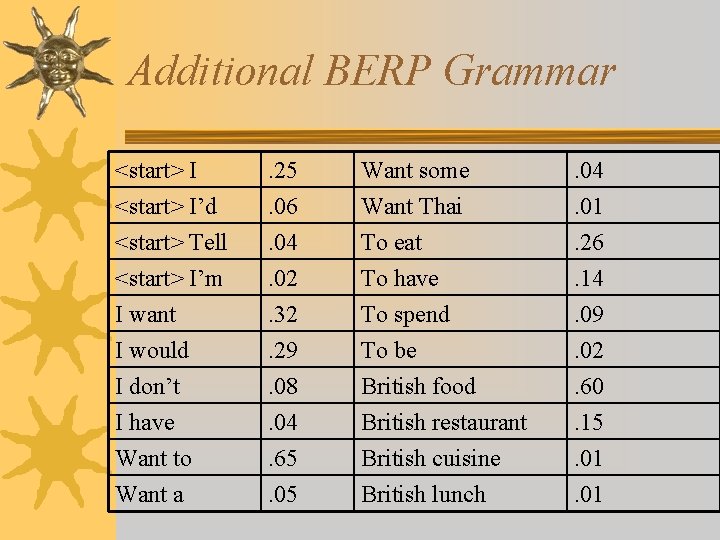
Additional BERP Grammar <start> I’d <start> Tell <start> I’m . 25. 06. 04. 02 Want some Want Thai To eat To have . 04. 01. 26. 14 I want I would I don’t I have Want to Want a . 32. 29. 08. 04. 65. 05 To spend To be British food British restaurant British cuisine British lunch . 09. 02. 60. 15. 01

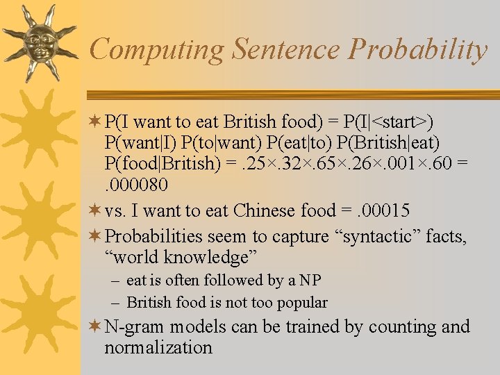
Computing Sentence Probability ¬ P(I want to eat British food) = P(I|<start>) P(want|I) P(to|want) P(eat|to) P(British|eat) P(food|British) =. 25×. 32×. 65×. 26×. 001×. 60 =. 000080 ¬ vs. I want to eat Chinese food =. 00015 ¬ Probabilities seem to capture “syntactic” facts, “world knowledge” – eat is often followed by a NP – British food is not too popular ¬ N-gram models can be trained by counting and normalization

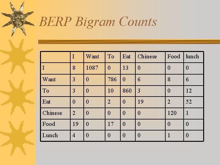
BERP Bigram Counts I Want To Eat Chinese Food lunch I 8 1087 0 13 0 0 0 Want 3 0 786 0 6 8 6 To 3 0 10 860 3 0 12 Eat 0 0 2 0 19 2 52 Chinese 2 0 0 120 1 Food 19 0 17 0 0 Lunch 4 0 0 1 0

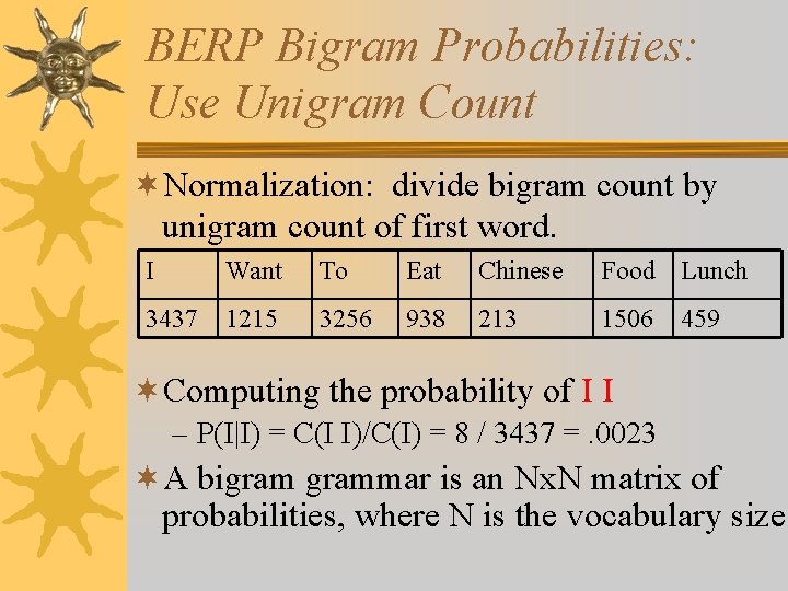
BERP Bigram Probabilities: Use Unigram Count ¬Normalization: divide bigram count by unigram count of first word. I Want To Eat Chinese Food Lunch 3437 1215 3256 938 213 1506 459 ¬Computing the probability of I I – P(I|I) = C(I I)/C(I) = 8 / 3437 =. 0023 ¬A bigrammar is an Nx. N matrix of probabilities, where N is the vocabulary size

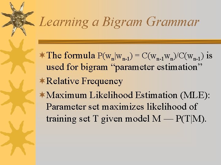
Learning a Bigram Grammar ¬The formula P(wn|wn-1) = C(wn-1 wn)/C(wn-1) is used for bigram “parameter estimation” ¬Relative Frequency ¬Maximum Likelihood Estimation (MLE): Parameter set maximizes likelihood of training set T given model M — P(T|M).

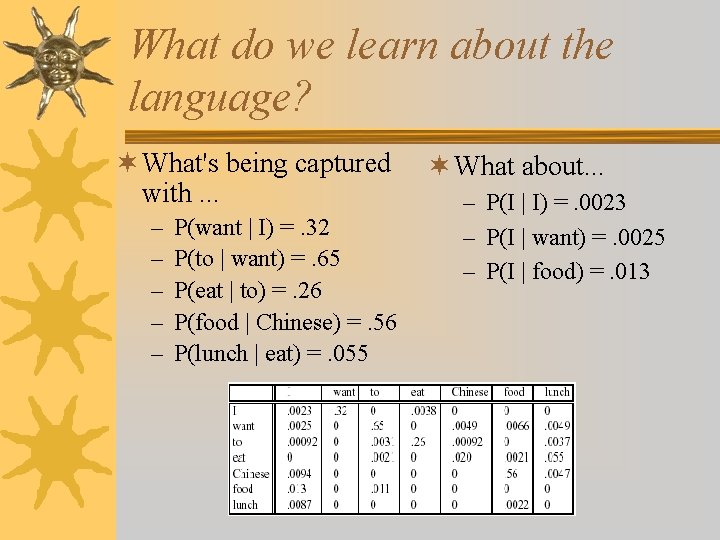
What do we learn about the language? ¬ What's being captured with. . . – – – P(want | I) =. 32 P(to | want) =. 65 P(eat | to) =. 26 P(food | Chinese) =. 56 P(lunch | eat) =. 055 ¬ What about. . . – P(I | I) =. 0023 – P(I | want) =. 0025 – P(I | food) =. 013

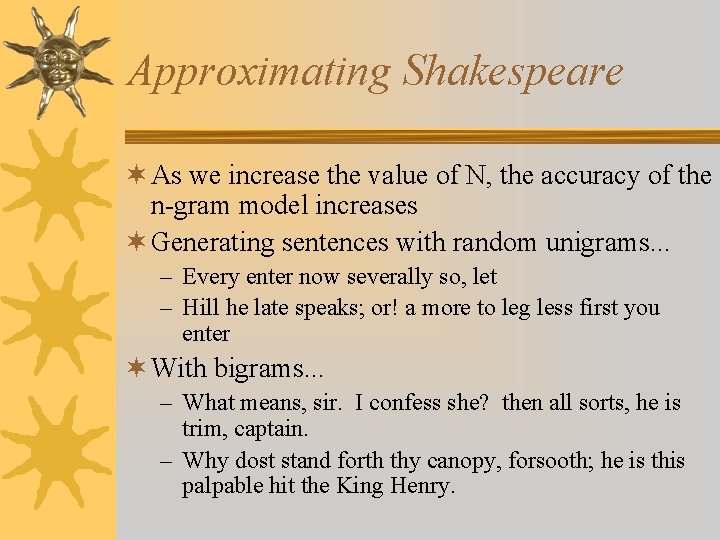
Approximating Shakespeare ¬ As we increase the value of N, the accuracy of the n-gram model increases ¬ Generating sentences with random unigrams. . . – Every enter now severally so, let – Hill he late speaks; or! a more to leg less first you enter ¬ With bigrams. . . – What means, sir. I confess she? then all sorts, he is trim, captain. – Why dost stand forth thy canopy, forsooth; he is this palpable hit the King Henry.

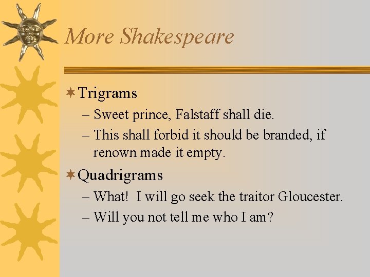
More Shakespeare ¬Trigrams – Sweet prince, Falstaff shall die. – This shall forbid it should be branded, if renown made it empty. ¬Quadrigrams – What! I will go seek the traitor Gloucester. – Will you not tell me who I am?

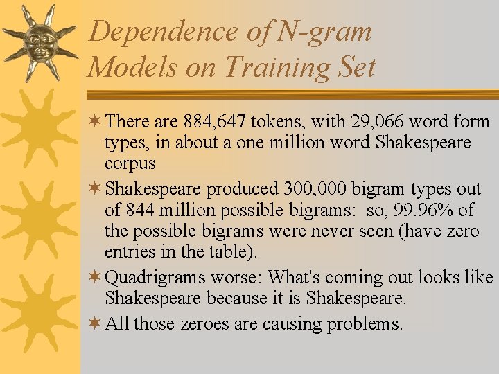
Dependence of N-gram Models on Training Set ¬ There are 884, 647 tokens, with 29, 066 word form types, in about a one million word Shakespeare corpus ¬ Shakespeare produced 300, 000 bigram types out of 844 million possible bigrams: so, 99. 96% of the possible bigrams were never seen (have zero entries in the table). ¬ Quadrigrams worse: What's coming out looks like Shakespeare because it is Shakespeare. ¬ All those zeroes are causing problems.

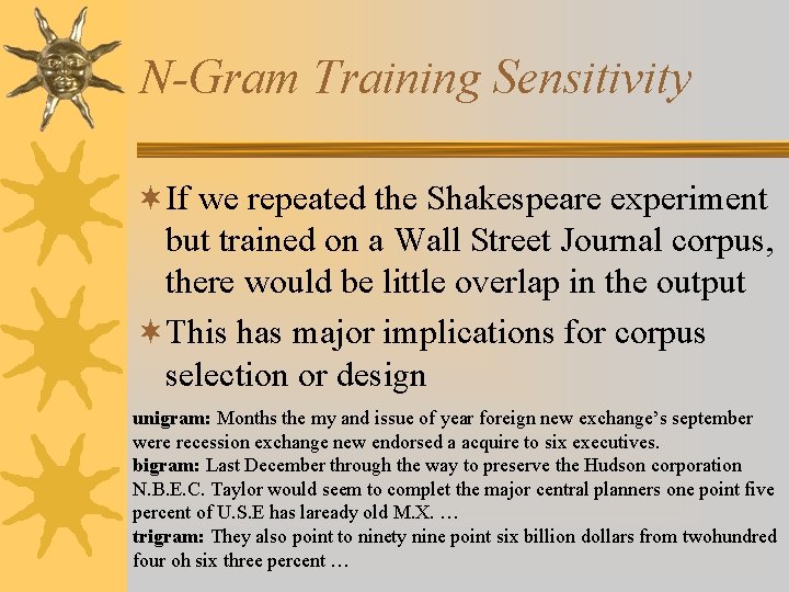
N-Gram Training Sensitivity ¬If we repeated the Shakespeare experiment but trained on a Wall Street Journal corpus, there would be little overlap in the output ¬This has major implications for corpus selection or design unigram: Months the my and issue of year foreign new exchange’s september were recession exchange new endorsed a acquire to six executives. bigram: Last December through the way to preserve the Hudson corporation N. B. E. C. Taylor would seem to complet the major central planners one point five percent of U. S. E has laready old M. X. … trigram: They also point to ninety nine point six billion dollars from twohundred four oh six three percent …

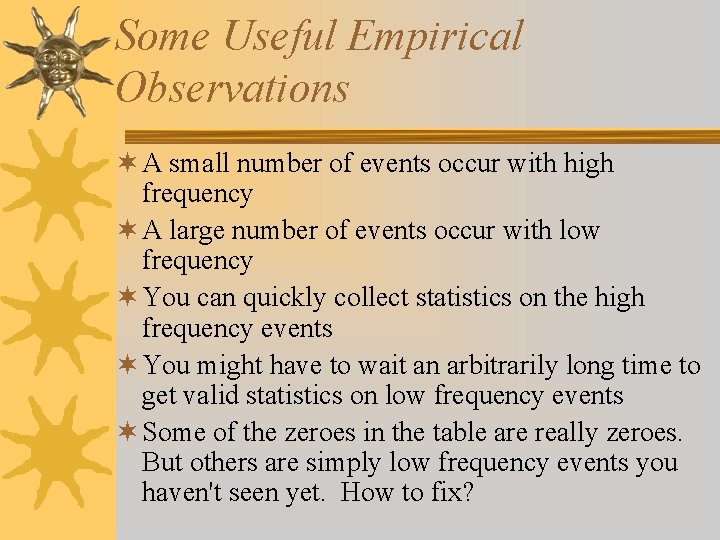
Some Useful Empirical Observations ¬ A small number of events occur with high frequency ¬ A large number of events occur with low frequency ¬ You can quickly collect statistics on the high frequency events ¬ You might have to wait an arbitrarily long time to get valid statistics on low frequency events ¬ Some of the zeroes in the table are really zeroes. But others are simply low frequency events you haven't seen yet. How to fix?

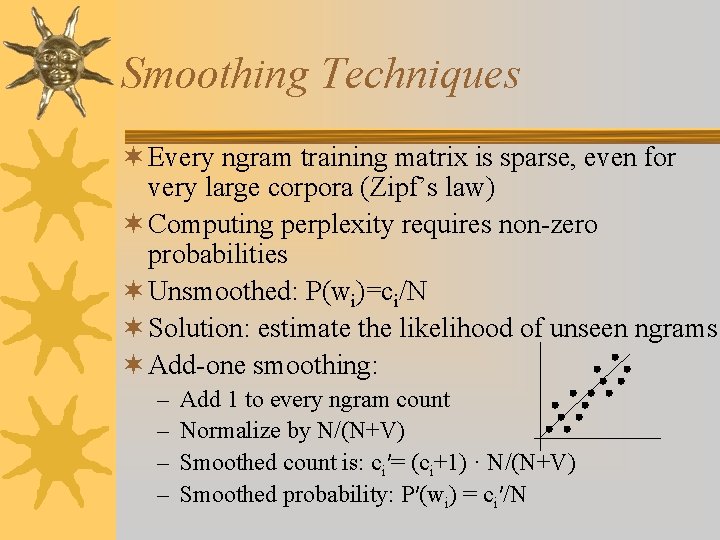
Smoothing Techniques ¬ Every ngram training matrix is sparse, even for very large corpora (Zipf’s law) ¬ Computing perplexity requires non-zero probabilities ¬ Unsmoothed: P(wi)=ci/N ¬ Solution: estimate the likelihood of unseen ngrams ¬ Add-one smoothing: – – Add 1 to every ngram count Normalize by N/(N+V) Smoothed count is: ci′= (ci+1) · N/(N+V) Smoothed probability: P′(wi) = ci′/N

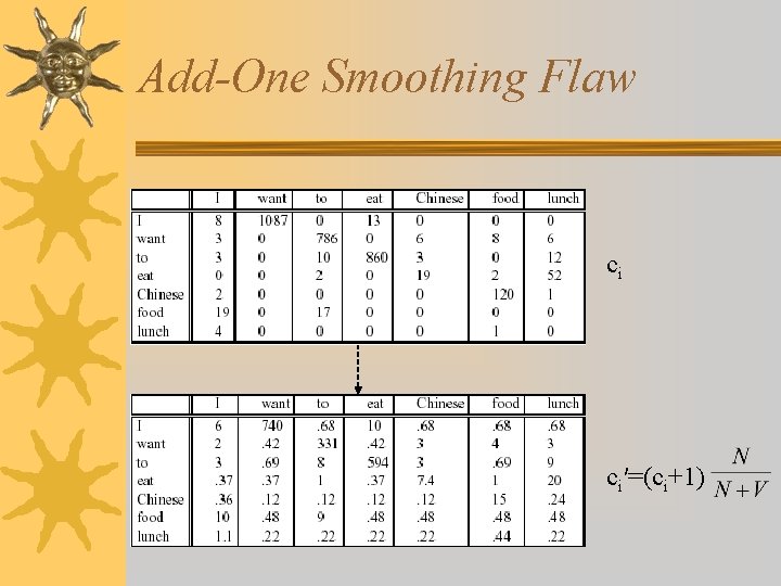
Add-One Smoothed Bigrams P(wn|wn-1) = C(wn-1 wn)/C(wn-1) P′(wn|wn-1) = [C(wn-1 wn)+1]/[C(wn-1)+V]

Add-One Smoothing Flaw ci ci′=(ci+1)

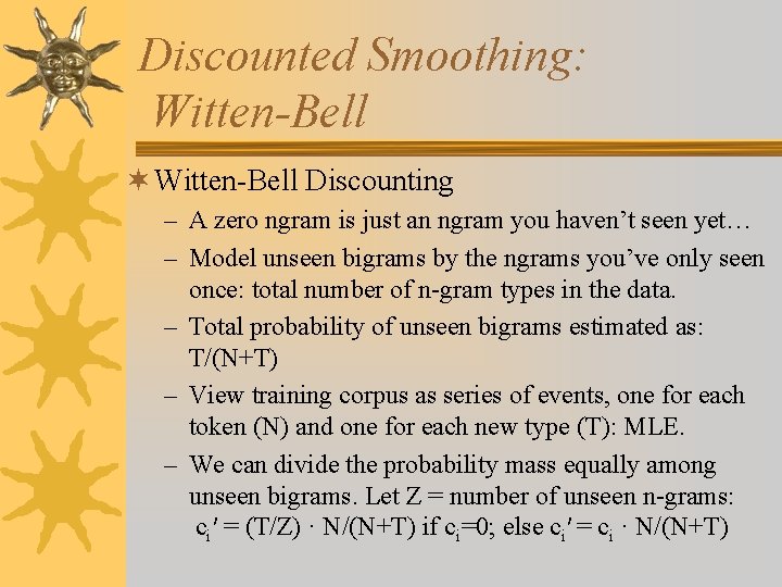
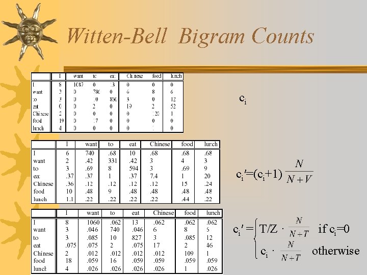
Discounted Smoothing: Witten-Bell ¬ Witten-Bell Discounting – A zero ngram is just an ngram you haven’t seen yet… – Model unseen bigrams by the ngrams you’ve only seen once: total number of n-gram types in the data. – Total probability of unseen bigrams estimated as: T/(N+T) – View training corpus as series of events, one for each token (N) and one for each new type (T): MLE. – We can divide the probability mass equally among unseen bigrams. Let Z = number of unseen n-grams: ci′ = (T/Z) · N/(N+T) if ci=0; else ci′ = ci · N/(N+T)

Witten-Bell Bigram Counts ci ci′=(ci+1) ci′ = T/Z · ci · if ci=0 otherwise

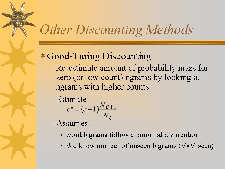
Other Discounting Methods ¬Good-Turing Discounting – Re-estimate amount of probability mass for zero (or low count) ngrams by looking at ngrams with higher counts – Estimate – Assumes: • word bigrams follow a binomial distribution • We know number of unseen bigrams (Vx. V-seen)

Readings for next time ¬J&M Chapter 7. 1 -7. 3