Chapter 9 Machine Independent Optimizations Data Flow Analysis

Chapter 9 Machine. Independent Optimizations

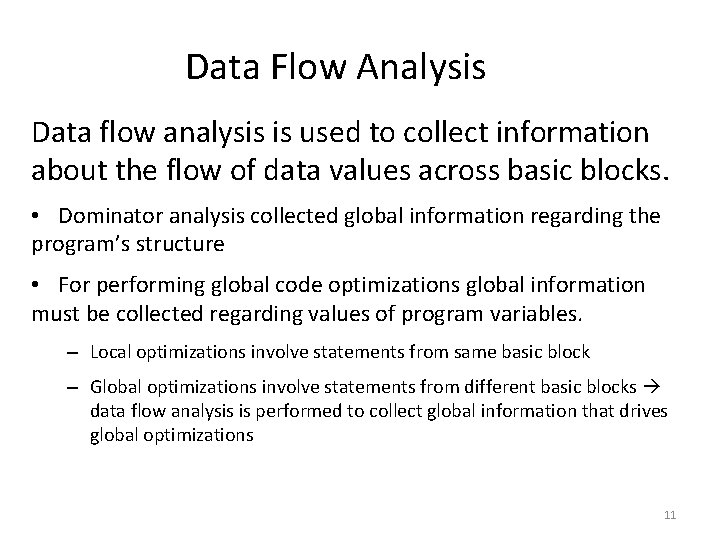
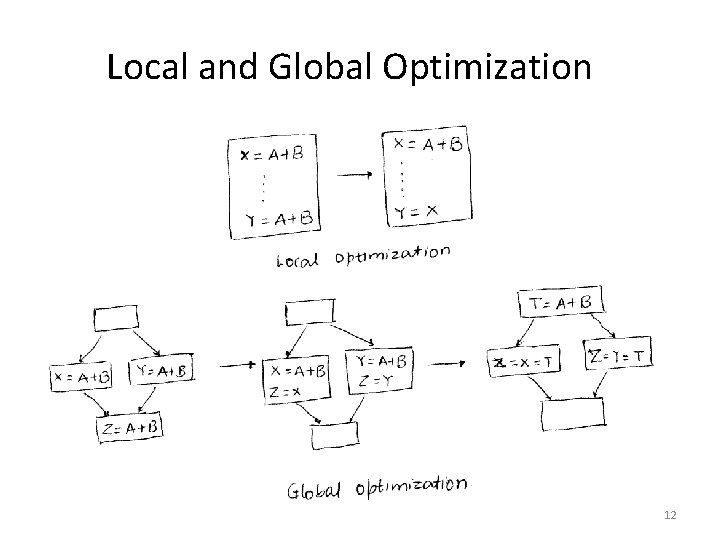
Data Flow Analysis Data flow analysis is used to collect information about the flow of data values across basic blocks. • Dominator analysis collected global information regarding the program’s structure • For performing global code optimizations global information must be collected regarding values of program variables. – Local optimizations involve statements from same basic block – Global optimizations involve statements from different basic blocks data flow analysis is performed to collect global information that drives global optimizations 11

Local and Global Optimization 12

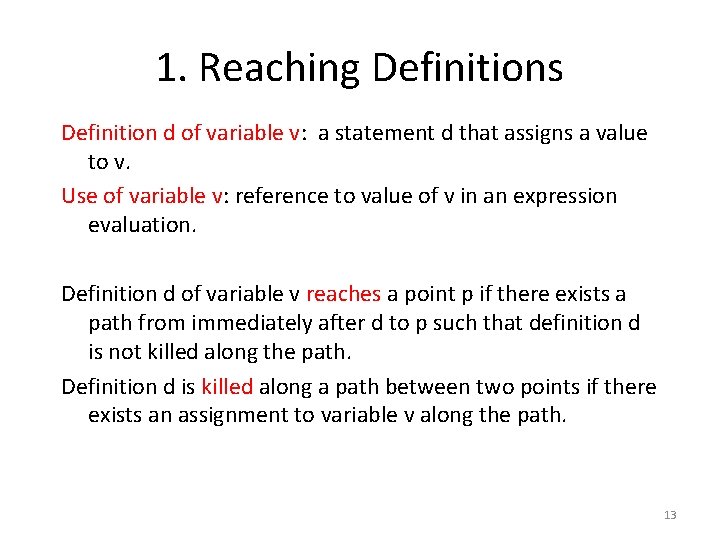
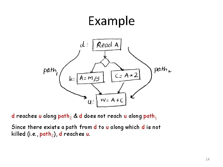
1. Reaching Definitions Definition d of variable v: a statement d that assigns a value to v. Use of variable v: reference to value of v in an expression evaluation. Definition d of variable v reaches a point p if there exists a path from immediately after d to p such that definition d is not killed along the path. Definition d is killed along a path between two points if there exists an assignment to variable v along the path. 13

Example d reaches u along path 2 & d does not reach u along path 1 Since there exists a path from d to u along which d is not killed (i. e. , path 2), d reaches u. 14

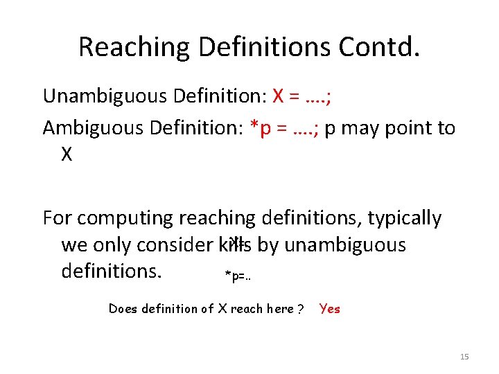
Reaching Definitions Contd. Unambiguous Definition: X = …. ; Ambiguous Definition: *p = …. ; p may point to X For computing reaching definitions, typically X=. . by unambiguous we only consider kills definitions. *p=. . Does definition of X reach here ? Yes 15

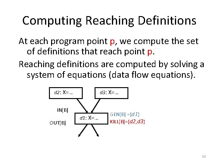
Computing Reaching Definitions At each program point p, we compute the set of definitions that reach point p. Reaching definitions are computed by solving a system of equations (data flow equations). d 2: X=… d 3: X=… IN[B] OUT[B] d 1: X=… GEN[B] ={d 1} KILL[B]={d 2, d 3} 16

Data Flow Equations IN[B]: Definitions that reach B’s entry. OUT[B]: Definitions that reach B’s exit. GEN[B]: Definitions within B that reach the end of B. KILL[B]: Definitions that never reach the end of B due to redefinitions of variables in B. 17

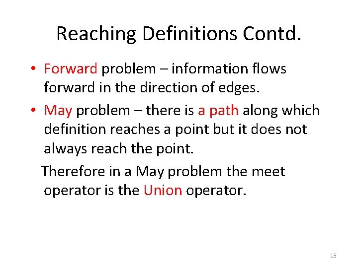
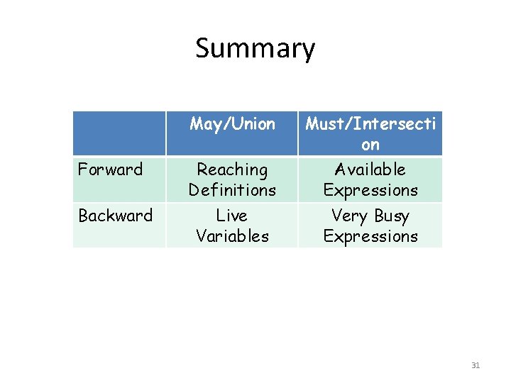
Reaching Definitions Contd. • Forward problem – information flows forward in the direction of edges. • May problem – there is a path along which definition reaches a point but it does not always reach the point. Therefore in a May problem the meet operator is the Union operator. 18

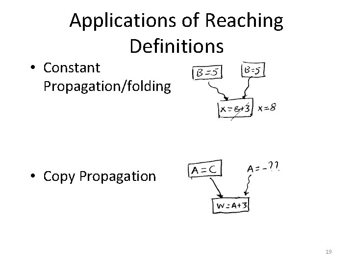
Applications of Reaching Definitions • Constant Propagation/folding • Copy Propagation 19

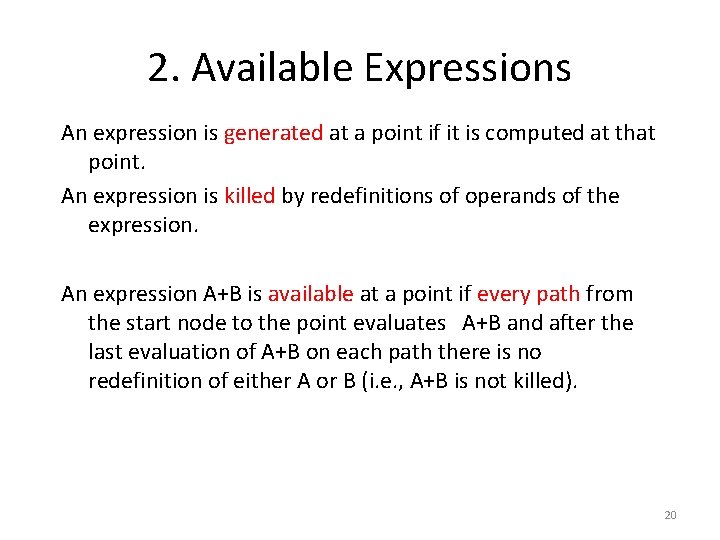
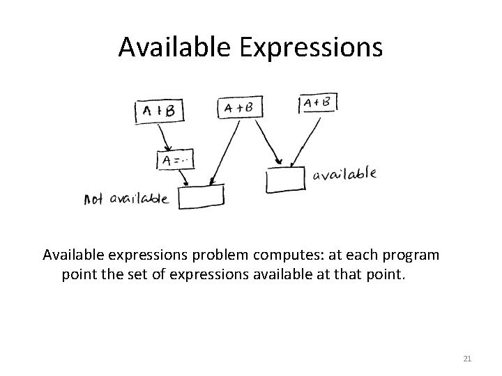
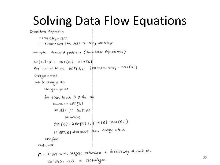
2. Available Expressions An expression is generated at a point if it is computed at that point. An expression is killed by redefinitions of operands of the expression. An expression A+B is available at a point if every path from the start node to the point evaluates A+B and after the last evaluation of A+B on each path there is no redefinition of either A or B (i. e. , A+B is not killed). 20

Available Expressions Available expressions problem computes: at each program point the set of expressions available at that point. 21

Data Flow Equations IN[B]: Expressions available at B’s entry. OUT[B]: Expressions available at B’s exit. GEN[B]: Expressions computed within B that are available at the end of B. KILL[B]: Expressions whose operands are redefined in B. 22

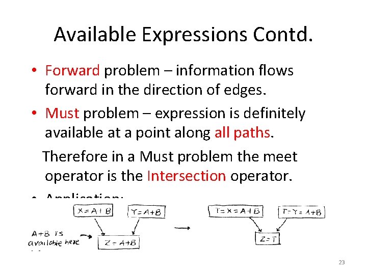
Available Expressions Contd. • Forward problem – information flows forward in the direction of edges. • Must problem – expression is definitely available at a point along all paths. Therefore in a Must problem the meet operator is the Intersection operator. • Application: A 23

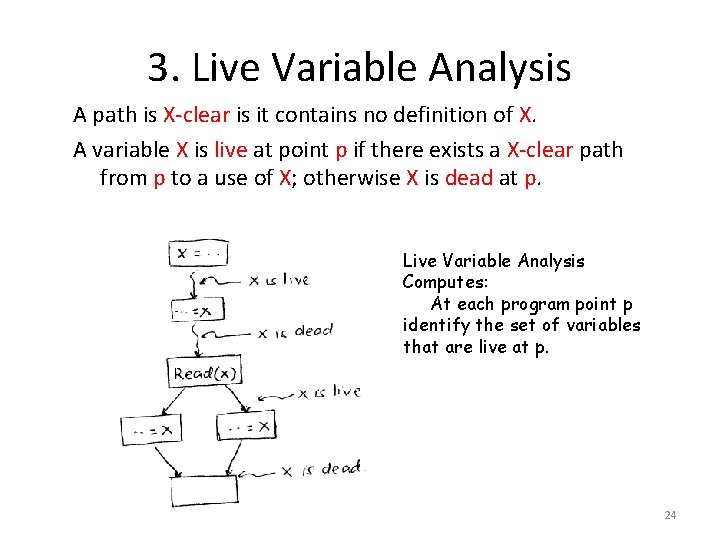
3. Live Variable Analysis A path is X-clear is it contains no definition of X. A variable X is live at point p if there exists a X-clear path from p to a use of X; otherwise X is dead at p. Live Variable Analysis Computes: At each program point p identify the set of variables that are live at p. 24

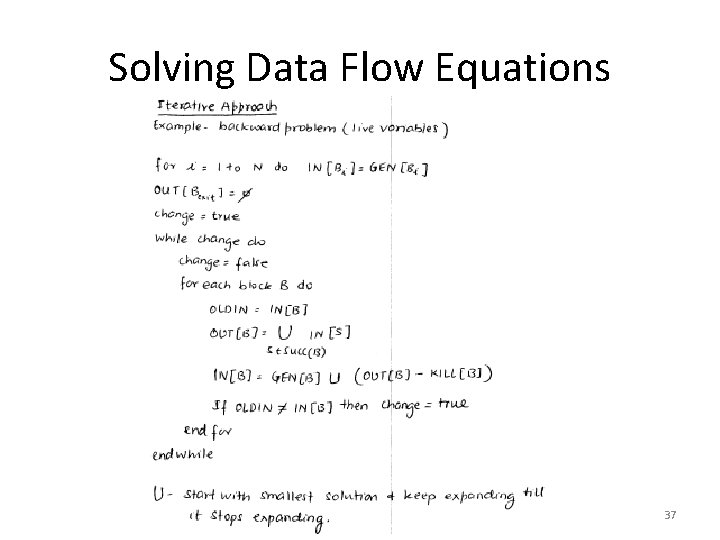
Data Flow Equations IN[B]: Variables live at B’s entry. OUT[B]: Variables live at B’s exit. GEN[B]: Variables that are used in B prior to their definition in B. KILL[B]: Variables definitely assigned value in B before any use of that variable in B. 25

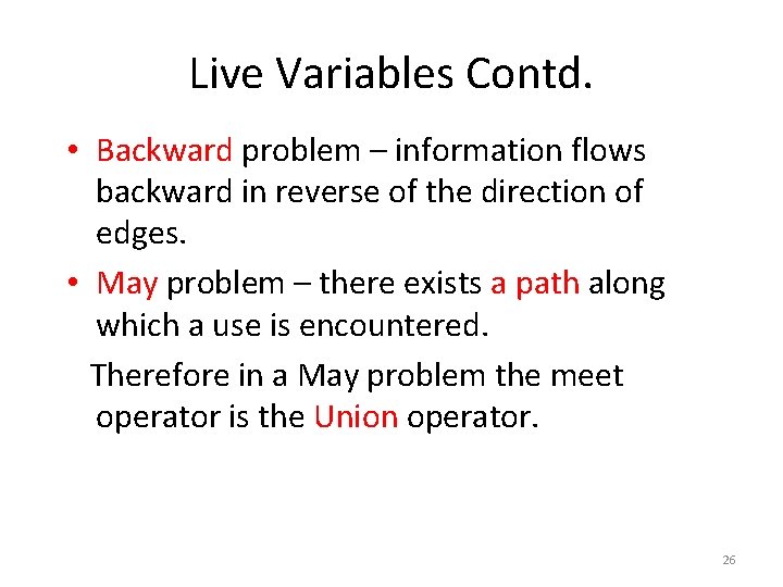
Live Variables Contd. • Backward problem – information flows backward in reverse of the direction of edges. • May problem – there exists a path along which a use is encountered. Therefore in a May problem the meet operator is the Union operator. 26

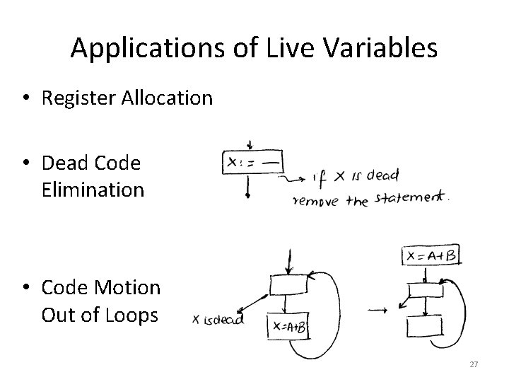
Applications of Live Variables • Register Allocation • Dead Code Elimination • Code Motion Out of Loops 27

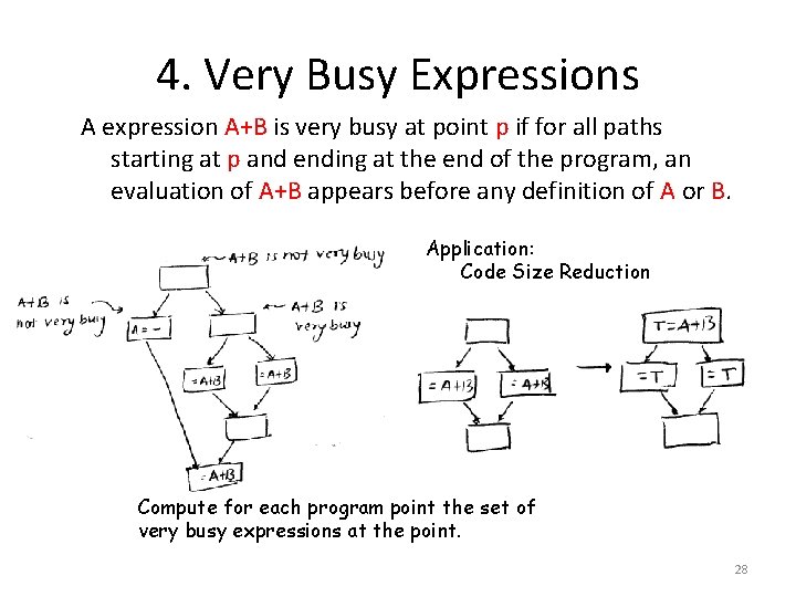
4. Very Busy Expressions A expression A+B is very busy at point p if for all paths starting at p and ending at the end of the program, an evaluation of A+B appears before any definition of A or B. Application: Code Size Reduction Compute for each program point the set of very busy expressions at the point. 28

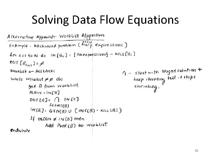
Data Flow Equations IN[B]: Expressions very busy at B’s entry. OUT[B]: Expressions very busy at B’s exit. GEN[B]: Expression computed in B and variables used in the expression are not redefined in B prior to expression’s evaluation in B. KILL[B]: Expressions that use variables that are redefined in B. 29

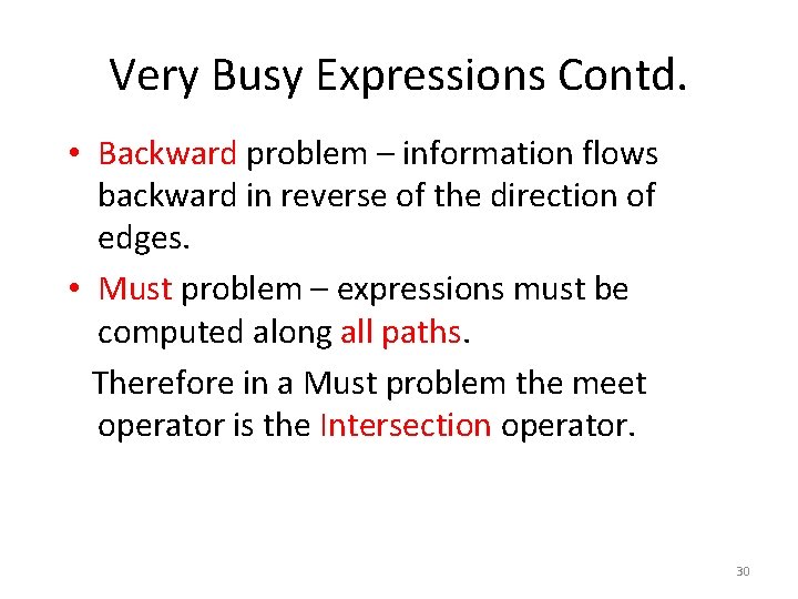
Very Busy Expressions Contd. • Backward problem – information flows backward in reverse of the direction of edges. • Must problem – expressions must be computed along all paths. Therefore in a Must problem the meet operator is the Intersection operator. 30

Summary May/Union Must/Intersecti on Forward Reaching Definitions Available Expressions Backward Live Variables Very Busy Expressions 31

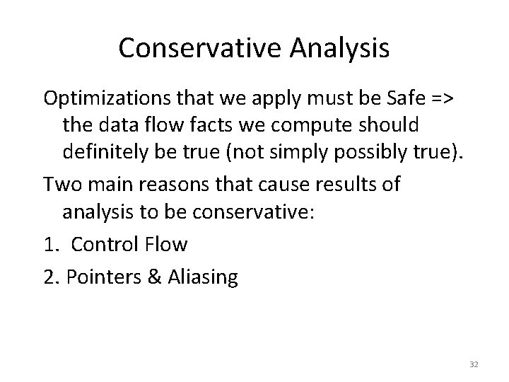
Conservative Analysis Optimizations that we apply must be Safe => the data flow facts we compute should definitely be true (not simply possibly true). Two main reasons that cause results of analysis to be conservative: 1. Control Flow 2. Pointers & Aliasing 32

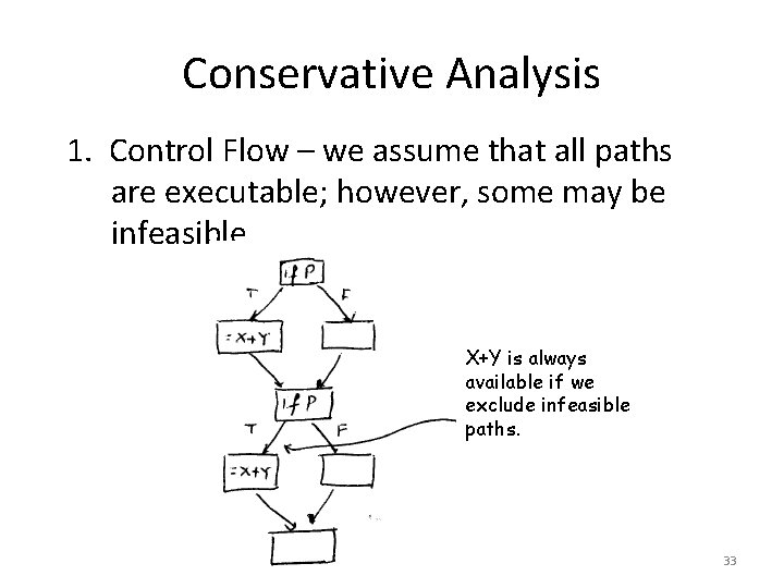
Conservative Analysis 1. Control Flow – we assume that all paths are executable; however, some may be infeasible. X+Y is always available if we exclude infeasible paths. 33

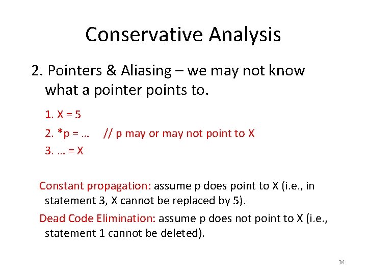
Conservative Analysis 2. Pointers & Aliasing – we may not know what a pointer points to. 1. X = 5 2. *p = … 3. … = X // p may or may not point to X Constant propagation: assume p does point to X (i. e. , in statement 3, X cannot be replaced by 5). Dead Code Elimination: assume p does not point to X (i. e. , statement 1 cannot be deleted). 34

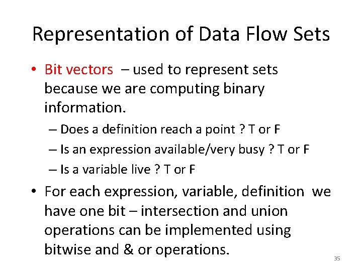
Representation of Data Flow Sets • Bit vectors – used to represent sets because we are computing binary information. – Does a definition reach a point ? T or F – Is an expression available/very busy ? T or F – Is a variable live ? T or F • For each expression, variable, definition we have one bit – intersection and union operations can be implemented using bitwise and & or operations. 35

Solving Data Flow Equations 36

Solving Data Flow Equations 37

Solving Data Flow Equations 38

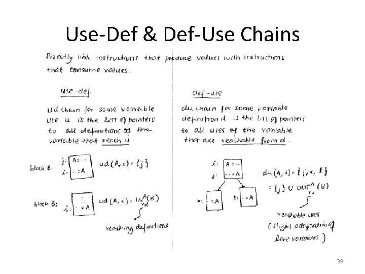
Use-Def & Def-Use Chains 39

Sample Problems Data Flow Analysis 40

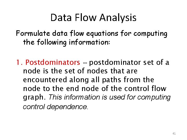
Data Flow Analysis Formulate data flow equations for computing the following information: 1. Postdominators -- postdominator set of a node is the set of nodes that are encountered along all paths from the node to the end node of the control flow graph. This information is used for computing control dependence. 41

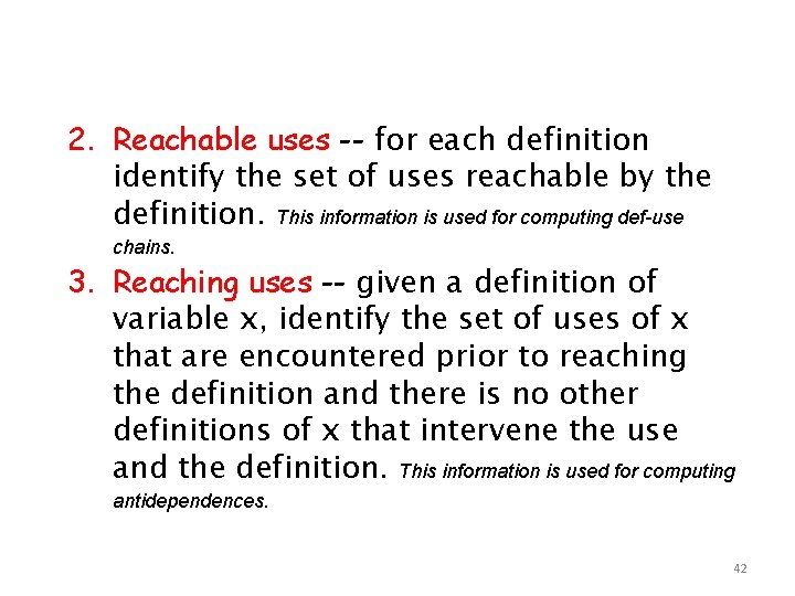
2. Reachable uses -- for each definition identify the set of uses reachable by the definition. This information is used for computing def-use chains. 3. Reaching uses -- given a definition of variable x, identify the set of uses of x that are encountered prior to reaching the definition and there is no other definitions of x that intervene the use and the definition. This information is used for computing antidependences. 42

4. Classify Variable Values -- classify the value of each program variable at each program point into one of the following categories: (a) the value is a unique constant -- you must also identify this constant value; (b) the value is one-of-many constants – you do not have to compute the identities of these constants as part of your solution; and (c) the value is not-a-constant, that is, it is neither a unique constant nor a one-ofmany constants. This is a generalization of constant propagation. 43