Course Topics Classical Compiler Optimizations and Control Flow

Course Topics • Classical Compiler Optimizations and Control Flow Graphs • Dataflow Analysis • • Software Testing Refactoring Type-based Analysis More…

Outline of Today’s Class • Local analysis vs. global analysis • Introduction to dataflow analysis • The four classical dataflow analysis problems – – Reaching definitions Live variables Available expressions Very busy expressions • Reading: Compilers: Principles, Techniques and Tools, by Aho, Lam, Sethi and Ullman, Chapter 9. 2��

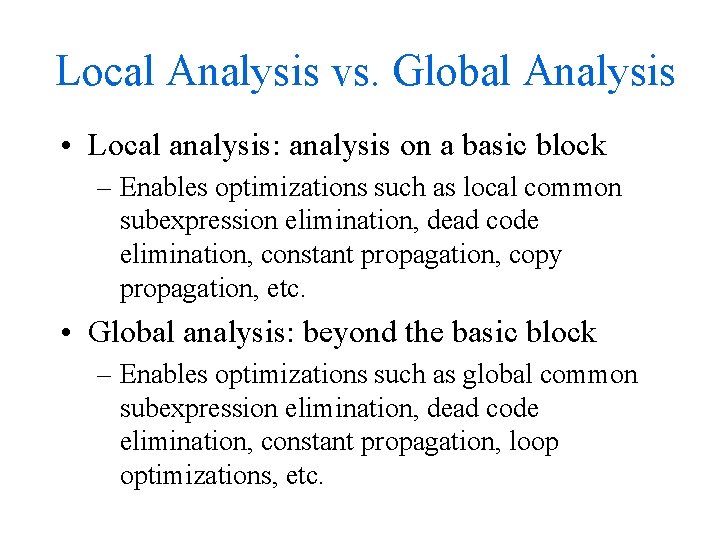
Local Analysis vs. Global Analysis • Local analysis: analysis on a basic block – Enables optimizations such as local common subexpression elimination, dead code elimination, constant propagation, copy propagation, etc. • Global analysis: beyond the basic block – Enables optimizations such as global common subexpression elimination, dead code elimination, constant propagation, loop optimizations, etc.

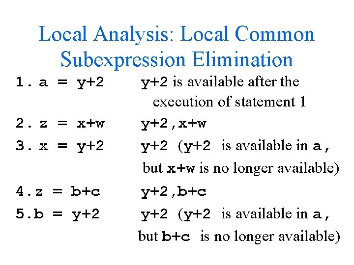
Local Analysis: Local Common Subexpression Elimination 1. a = y+2 2. z = x+w 3. x = y+2 4. z = b+c 5. b = y+2 is available after the execution of statement 1 y+2, x+w y+2 (y+2 is available in a, but x+w is no longer available) y+2, b+c y+2 (y+2 is available in a, but b+c is no longer available)

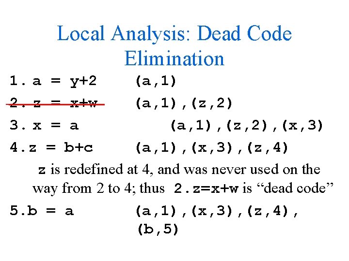
Local Analysis: Dead Code Elimination 1. a = y+2 (a, 1) 2. z = x+w (a, 1), (z, 2) 3. x = a (a, 1), (z, 2), (x, 3) 4. z = b+c (a, 1), (x, 3), (z, 4) z is redefined at 4, and was never used on the way from 2 to 4; thus 2. z=x+w is “dead code” 5. b = a (a, 1), (x, 3), (z, 4), (b, 5)

Local Analysis vs. Global Analysis • Local analysis is easy – we need to take into account a single path, from basic block entry to basic block exit • Global analysis is harder – we need to take into account multiple paths, across basic blocks

Introduction to Dataflow Analysis • Collects information about the flow of data along all paths� – Loops (control goes back) – Control splits and control merges • We can define many different kinds of dataflow analysis

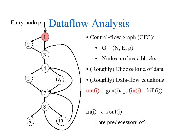
Dataflow Analysis Entry node ρ: • Control-flow graph (CFG): 1 2 • G = (N, E, ρ) 3 • Nodes are basic blocks 4 5 • (Roughly) Choose kind of data 6 out(i) = gen(i) 7 8 9 • (Roughly) Data-flow equations in(i) = 10 (in(i) – kill(i)) out(j) j are predecessors of i

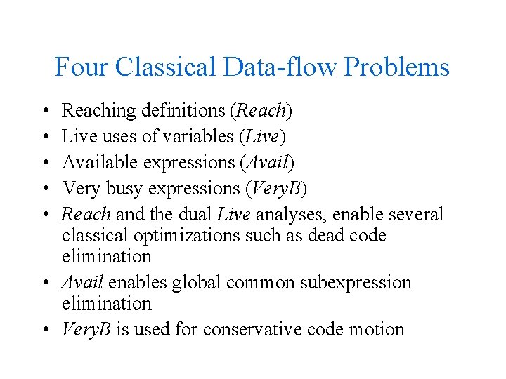
Four Classical Data-flow Problems • • • Reaching definitions (Reach) Live uses of variables (Live) Available expressions (Avail) Very busy expressions (Very. B) Reach and the dual Live analyses, enable several classical optimizations such as dead code elimination • Avail enables global common subexpression elimination • Very. B is used for conservative code motion

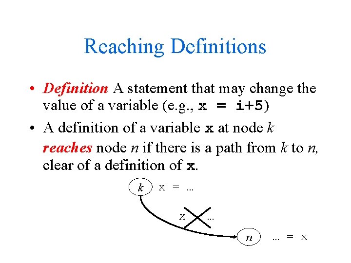
Reaching Definitions • Definition A statement that may change the value of a variable (e. g. , x = i+5) • A definition of a variable x at node k reaches node n if there is a path from k to n, clear of a definition of x. k x = … n … = x

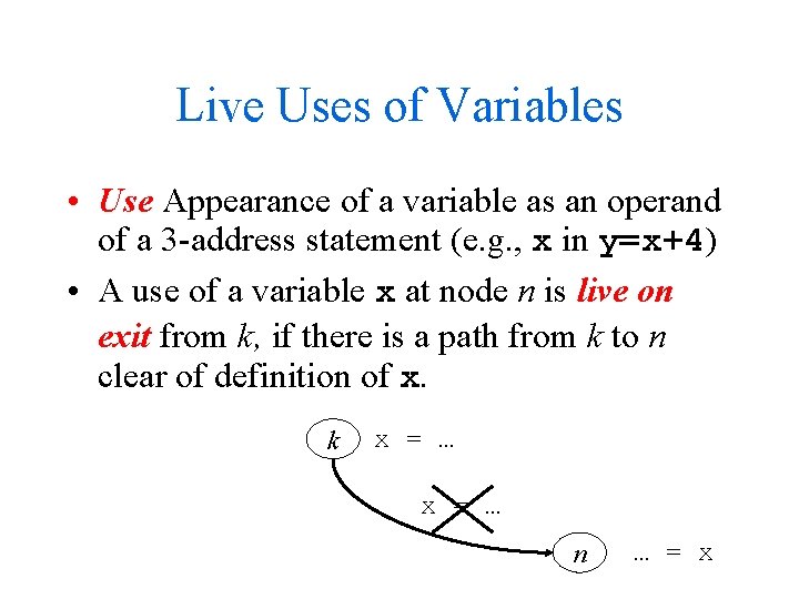
Live Uses of Variables • Use Appearance of a variable as an operand of a 3 -address statement (e. g. , x in y=x+4) • A use of a variable x at node n is live on exit from k, if there is a path from k to n clear of definition of x. k x = … n … = x

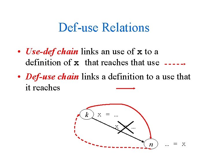
Def-use Relations • Use-def chain links an use of x to a definition of x that reaches that use • Def-use chain links a definition to a use that it reaches k x = … n … = x

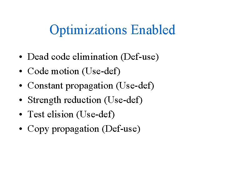
Optimizations Enabled • • • Dead code elimination (Def-use) Code motion (Use-def) Constant propagation (Use-def) Strength reduction (Use-def) Test elision (Use-def) Copy propagation (Def-use)

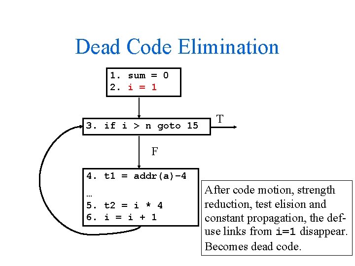
Dead Code Elimination 1. sum = 0 2. i = 1 3. if i > n goto 15 T F 4. t 1 = addr(a)– 4 … 5. t 2 = i * 4 6. i = i + 1 After code motion, strength reduction, test elision and constant propagation, the defuse links from i=1 disappear. Becomes dead code.

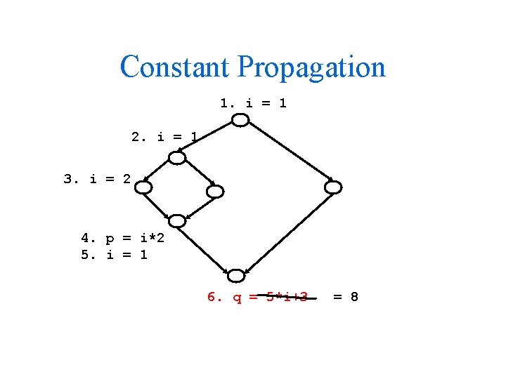
Constant Propagation 1. i = 1 2. i = 1 3. i = 2 4. p = i*2 5. i = 1 6. q = 5*i+3 = 8

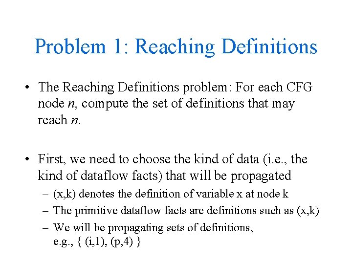
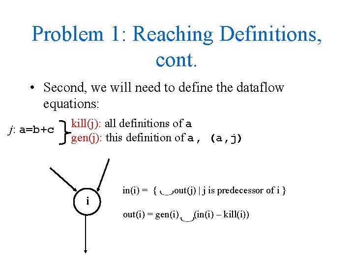
Problem 1: Reaching Definitions • The Reaching Definitions problem: For each CFG node n, compute the set of definitions that may reach n. • First, we need to choose the kind of data (i. e. , the kind of dataflow facts) that will be propagated – (x, k) denotes the definition of variable x at node k – The primitive dataflow facts are definitions such as (x, k) – We will be propagating sets of definitions, e. g. , { (i, 1), (p, 4) }

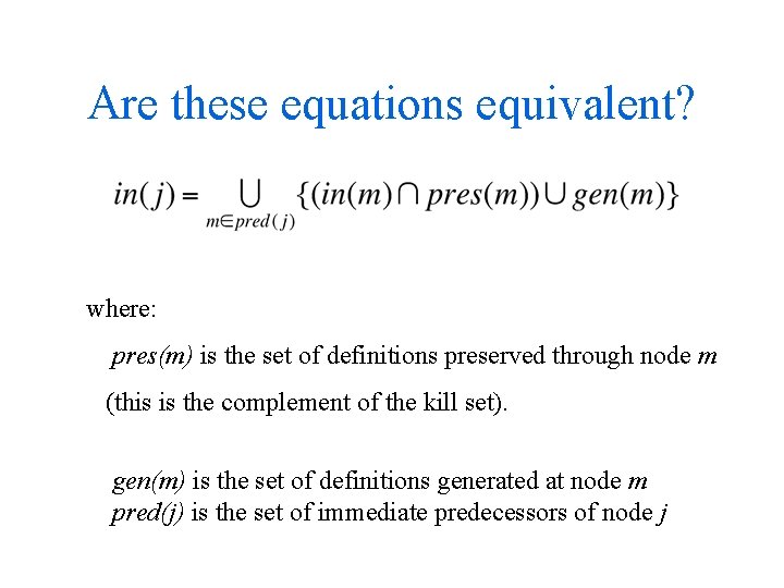
Problem 1: Reaching Definitions, cont. • Second, we will need to define the dataflow equations: j: a=b+c kill(j): all definitions of a gen(j): this definition of a, (a, j) i in(i) = { out(j) | j is predecessor of i } out(i) = gen(i) (in(i) – kill(i))

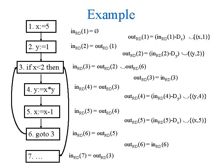
Example 1. x: =5 in. RD(1) = Ø 2. y: =1 in. RD(2) = out. RD (1) 3. if x<2 then in. RD(3) = out. RD(2) out. RD(1) = (in. RD(1)-Dx) out. RD(2) = (in. RD(2)-Dy) {(x, 1)} {(y, 2)} out. RD(6) out. RD(3) = in. RD(3) 4. y: =x*y in. RD(4) = out. RD(3) 5. x: =x-1 in. RD(5) = out. RD(4) 6. goto 3 out. RD(4) = (in. RD(4)-Dy) {(y, 4)} out. RD(5) = (in. RD(5)-Dx) {(x, 5)} in. RD(6) = out. RD(5) out. RD(6) = in. RD(6) 7. … in. RD(7) = out. RD(3)

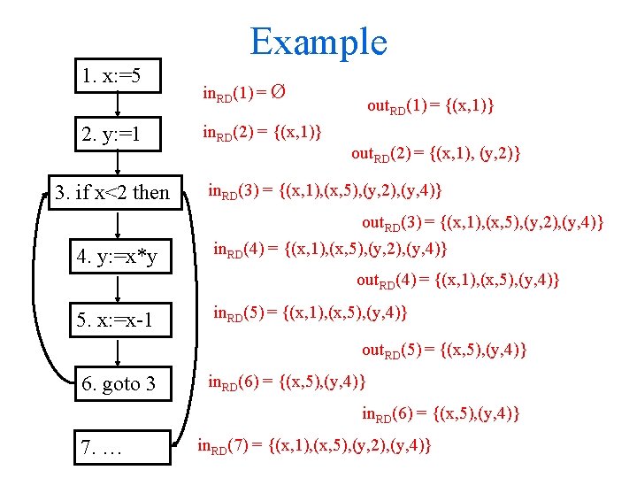
Example 1. x: =5 2. y: =1 3. if x<2 then in. RD(1) = Ø in. RD(2) = {(x, 1)} out. RD(1) = {(x, 1)} out. RD(2) = {(x, 1), (y, 2)} in. RD(3) = {(x, 1), (x, 5), (y, 2), (y, 4)} out. RD(3) = {(x, 1), (x, 5), (y, 2), (y, 4)} 4. y: =x*y in. RD(4) = {(x, 1), (x, 5), (y, 2), (y, 4)} out. RD(4) = {(x, 1), (x, 5), (y, 4)} 5. x: =x-1 in. RD(5) = {(x, 1), (x, 5), (y, 4)} out. RD(5) = {(x, 5), (y, 4)} 6. goto 3 in. RD(6) = {(x, 5), (y, 4)} 7. … in. RD(7) = {(x, 1), (x, 5), (y, 2), (y, 4)}

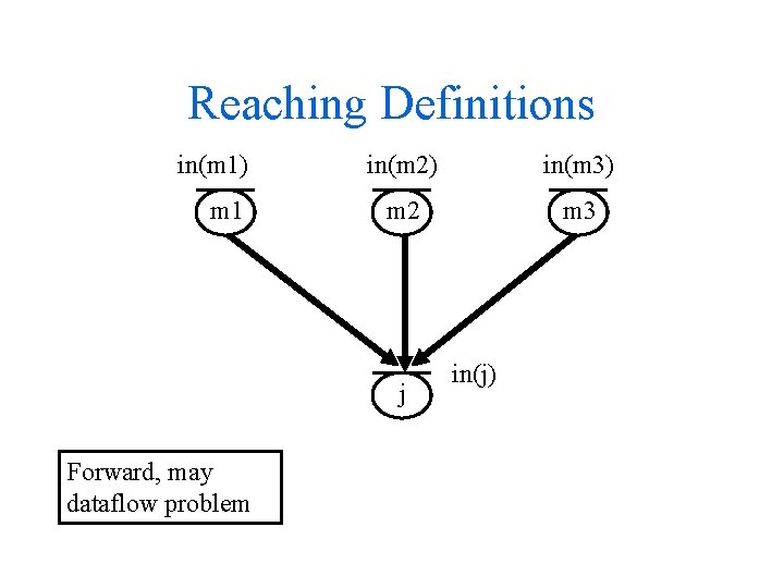
Reaching Definitions in(m 1) m 1 in(m 2) in(m 3) m 2 m 3 j Forward, may dataflow problem in(j)

Are these equations equivalent? where: pres(m) is the set of definitions preserved through node m (this is the complement of the kill set). gen(m) is the set of definitions generated at node m pred(j) is the set of immediate predecessors of node j