Chapter 5 The Standard Deviation as a Ruler

Chapter 5 The Standard Deviation as a Ruler and the Normal Model

The Standard Deviation as a Ruler • Now we are going to compare individual values with other data. • The trick in comparing very different-looking values is to use standard deviations as our rulers. • The standard deviation tells us how the whole collection of values varies, so it is a good way to compare an individual to a group.

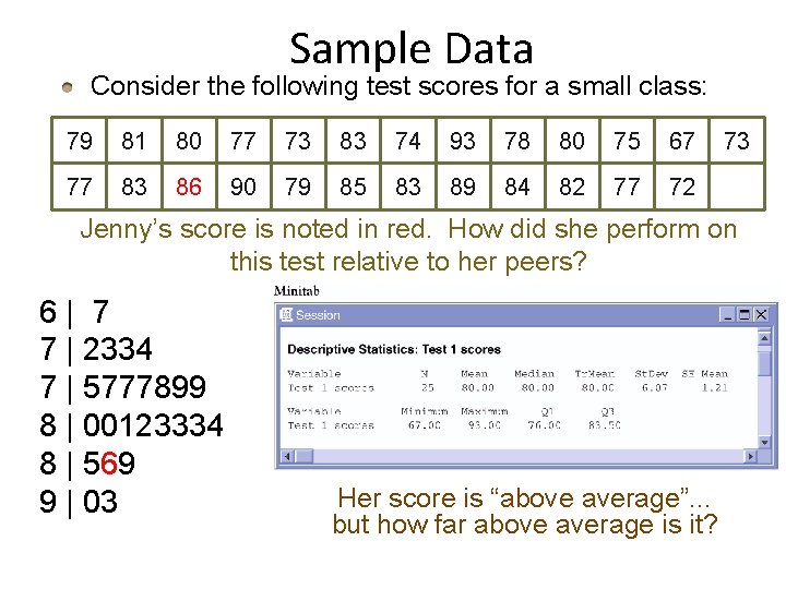
Sample Data Consider the following test scores for a small class: 79 81 80 77 73 83 74 93 78 80 75 67 77 83 86 90 79 85 83 89 84 82 77 72 73 Jenny’s score is noted in red. How did she perform on this test relative to her peers? 6| 7 7 | 2334 7 | 5777899 8 | 00123334 8 | 569 9 | 03 Her score is “above average”. . . but how far above average is it?

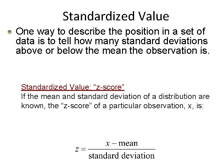
Standardized Value One way to describe the position in a set of data is to tell how many standard deviations above or below the mean the observation is. Standardized Value: “z-score” If the mean and standard deviation of a distribution are known, the “z-score” of a particular observation, x, is:

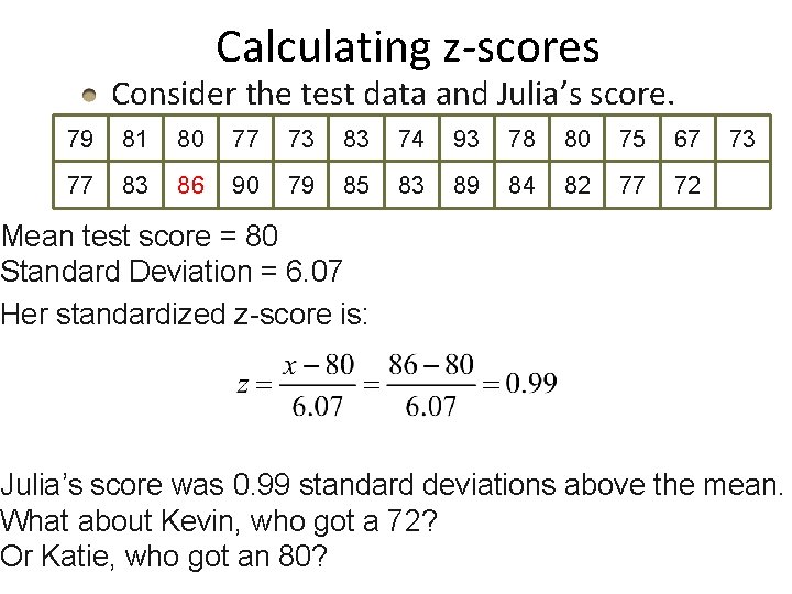
Calculating z-scores Consider the test data and Julia’s score. 79 81 80 77 73 83 74 93 78 80 75 67 77 83 86 90 79 85 83 89 84 82 77 72 73 Mean test score = 80 Standard Deviation = 6. 07 Her standardized z-score is: Julia’s score was 0. 99 standard deviations above the mean. What about Kevin, who got a 72? Or Katie, who got an 80?

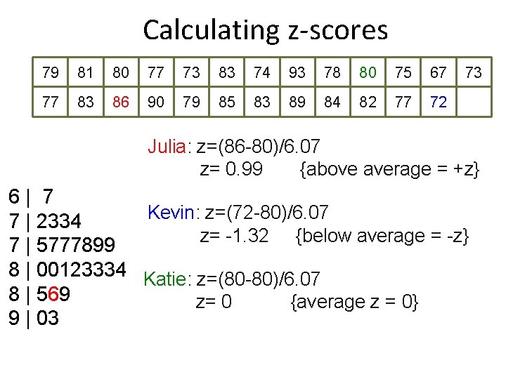
Calculating z-scores 79 81 80 77 73 83 74 93 78 80 75 67 77 83 86 90 79 85 83 89 84 82 77 72 73 Julia: z=(86 -80)/6. 07 z= 0. 99 {above average = +z} 6| 7 Kevin: z=(72 -80)/6. 07 7 | 2334 z= -1. 32 {below average = -z} 7 | 5777899 8 | 00123334 Katie: z=(80 -80)/6. 07 8 | 569 z= 0 {average z = 0} 9 | 03

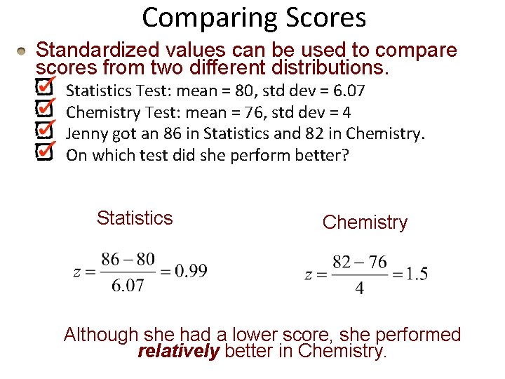
Comparing Scores Standardized values can be used to compare scores from two different distributions. Statistics Test: mean = 80, std dev = 6. 07 Chemistry Test: mean = 76, std dev = 4 Jenny got an 86 in Statistics and 82 in Chemistry. On which test did she perform better? Statistics Chemistry Although she had a lower score, she performed relatively better in Chemistry.

Standardizing with z-scores (cont. ) Note: • Standardized values have no units. • z-scores measure the distance of each data value from the mean in standard deviations. • A negative z-score tells us that the data value is below the mean • A positive z-score tells us that the data value is above the mean.

Benefits of Standardizing • Standardized values have been converted from their original units to the standard statistical unit of standard deviations from the mean. • This allows us to compare values that are measured on different scales, with different units, or from different populations.

Classwork: Z-Scores Worksheet

Homework: • Read Chapter 5 • Complete the Guided Reading

Shifting Data • Shifting data: – What would adding (or subtracting) a constant amount to each value do to the mean? – It would adds (or subtracts) the same constant to (from) the mean.

Shifting Data • Shifting data: – What would adding (or subtracting) a constant amount to each value do to the median or any other measure of position? – How would it effect the measures of spread? Adding a constant to every data value adds the same constant to measures of center and percentiles, but leaves measures of spread unchanged.

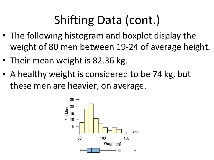
Shifting Data (cont. ) • The following histogram and boxplot display the weight of 80 men between 19 -24 of average height. • Their mean weight is 82. 36 kg. • A healthy weight is considered to be 74 kg, but these men are heavier, on average.

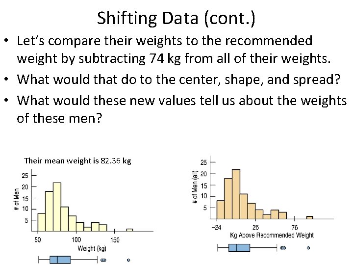
Shifting Data (cont. ) • Let’s compare their weights to the recommended weight by subtracting 74 kg from all of their weights. • What would that do to the center, shape, and spread? • What would these new values tell us about the weights of these men? Their mean weight is 82. 36 kg

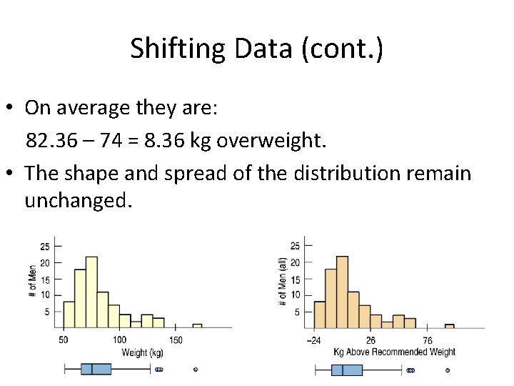
Shifting Data (cont. ) • On average they are: 82. 36 – 74 = 8. 36 kg overweight. • The shape and spread of the distribution remain unchanged.

Rescaling Data • Rescaling data: – When we divide or multiply all the data values by any constant value, what happens to all measures of position (such as the mean, median and percentiles)? – They are divided and multiplied by that same constant value.

Rescaling Data • Rescaling data: – When we divide or multiply all the data values by any constant value, what happens measures of spread (such as the range, IQR, and standard deviation)? – They are divided and multiplied by that same constant value.

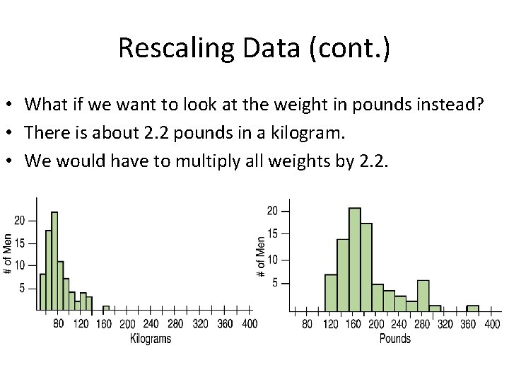
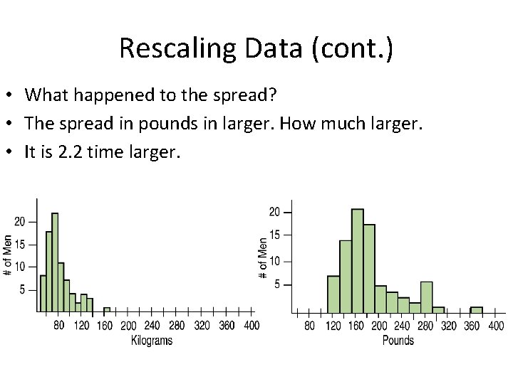
Rescaling Data (cont. ) • What if we want to look at the weight in pounds instead? • There is about 2. 2 pounds in a kilogram. • We would have to multiply all weights by 2. 2.

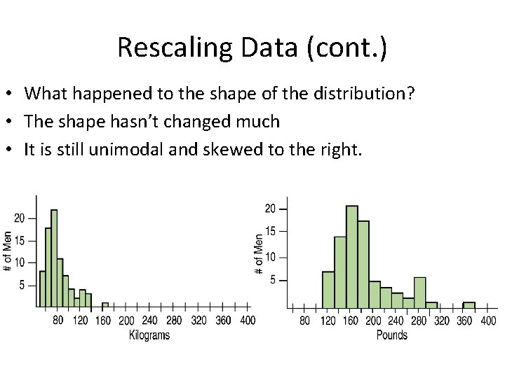
Rescaling Data (cont. ) • What happened to the shape of the distribution? • The shape hasn’t changed much • It is still unimodal and skewed to the right.

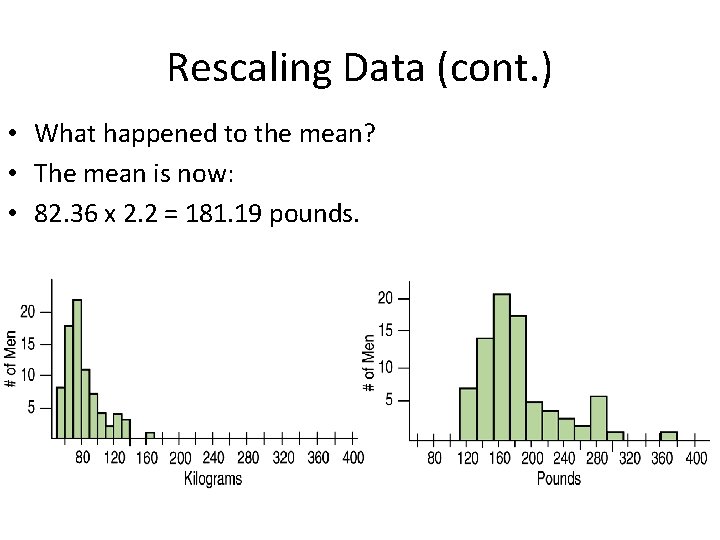
Rescaling Data (cont. ) • What happened to the mean? • The mean is now: • 82. 36 x 2. 2 = 181. 19 pounds.

Rescaling Data (cont. ) • What happened to the spread? • The spread in pounds in larger. How much larger. • It is 2. 2 time larger.

Back to z-scores • Standardizing data into z-scores shifts the data by subtracting the mean and rescales the values by dividing by their standard deviation. – Standardizing into z-scores does not change the shape of the distribution. – When we standardize into z-scores, this changes the center by making the mean equal to what? ZERO – When we standardize into z-scores, this changes the spread by making the standard deviation equal to what? ONE

Remember: Z-scores have a mean of 0 and a standard deviation of 1!

Classwork: Shifting and Rescaling Data Worksheet

Homework: • Chapter 4 Frappy • Read Chapter 5 • Complete the Guided Reading

When Is a z-score BIG? • A z-score gives us an indication of how unusual a value is because it tells us how far it is from the mean. • A data value that sits right at the mean, has a z-score equal to 0. • A z-score of 1 means the data value is 1 standard deviation above the mean. • A z-score of – 1 means the data value is 1 standard deviation below the mean.

When Is a z-score BIG? • How far from 0 does a z-score have to be interesting or unusual? • There is no universal standard, but the larger a z-score is (negative or positive), the more unusual it is.

When Is a z-score Big? (cont. ) • There is a model for z-scores that shows up over and over in Statistics. • This model is called the Normal model (You may have heard of “bell-shaped curves. ”). • Normal models are appropriate for distributions whose shapes are unimodal and roughly symmetric. • These distributions provide a measure of how extreme a z-score is.

When Is a z-score Big? (cont. ) • There is a Normal model for every possible combination of mean and standard deviation. – We write N(μ, σ) to represent a Normal model with a mean of μ and a standard deviation of σ. • We use Greek letters because this mean and standard deviation are not numerical summaries of the data. • They are numbers that we choose to help specify the model. • Such numbers are called parameters of the model.

Statistics vs. Parameters summarize the Population. (Use Greek letters for Parameters). Statistics summarize data from Samples.

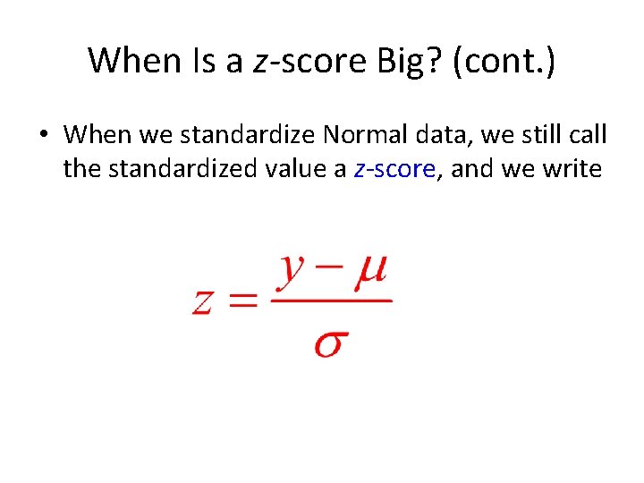
When Is a z-score Big? (cont. ) • When we standardize Normal data, we still call the standardized value a z-score, and we write

When Is a z-score Big? (cont. ) • Once we have standardized, we need only one model: – The N(0, 1) model is called the standard Normal model (or the standard Normal distribution). – It has a mean of 0 and a standard deviation of 1. • Be careful—don’t use a Normal model for just any data set, since standardizing does not change the shape of the distribution. • If the distribution is not unimodal and symmetric to begin with, standardizing won’t make it Normal.

When Is a z-score Big? (cont. ) • When we use the Normal model, we are assuming the distribution is Normal. • We cannot check this assumption in practice, so we check the following condition: – Nearly Normal Condition: The shape of the data’s distribution is unimodal and symmetric. – This condition can be checked with a histogram or a Normal probability plot (to be explained later).

The 68 -95 -99. 7 Rule • Normal models give us an idea of how extreme a value is by telling us how likely it is to find one that far from the mean.

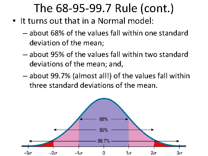
The 68 -95 -99. 7 Rule (cont. ) • It turns out that in a Normal model: – about 68% of the values fall within one standard deviation of the mean; – about 95% of the values fall within two standard deviations of the mean; and, – about 99. 7% (almost all!) of the values fall within three standard deviations of the mean.

Classwork/Homework: Drawing the Normal Model Worksheet Video (AP Stats Guy): https: //www. youtube. com/watch? feature=player_deta ilpage&v=xgolp. Gr. AZWo AP* Statistics – Classwork (Life Expectancy)

Homework: 1. Quiz on Drawing the Normal Model 2. Continue Reading Chapter 5 3. Work on Guided Reading

The First Three Rules for Working with Normal Models • Make a picture. • These still apply!!! • Drawing these help us think about the data’s distribution. • With data, make a histogram to check the Nearly Normal Condition.

Finding Normal Percentiles by Hand • What about when data value doesn’t fall exactly 1, 2, or 3 standard deviations from the mean? • We can look it up in a table of Normal percentiles or use technology. • Table Z in Appendix G provides us with normal percentiles.

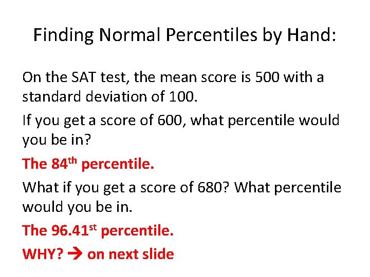
Finding Normal Percentiles by Hand: On the SAT test, the mean score is 500 with a standard deviation of 100. If you get a score of 600, what percentile would you be in? The 84 th percentile. What if you get a score of 680? What percentile would you be in. The 96. 41 st percentile. WHY? on next slide

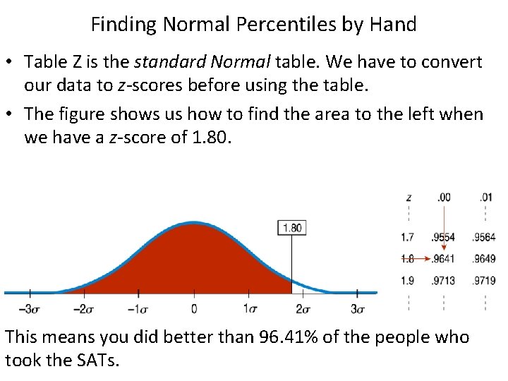
Finding Normal Percentiles by Hand • Table Z is the standard Normal table. We have to convert our data to z-scores before using the table. • The figure shows us how to find the area to the left when we have a z-score of 1. 80. This means you did better than 96. 41% of the people who took the SATs.

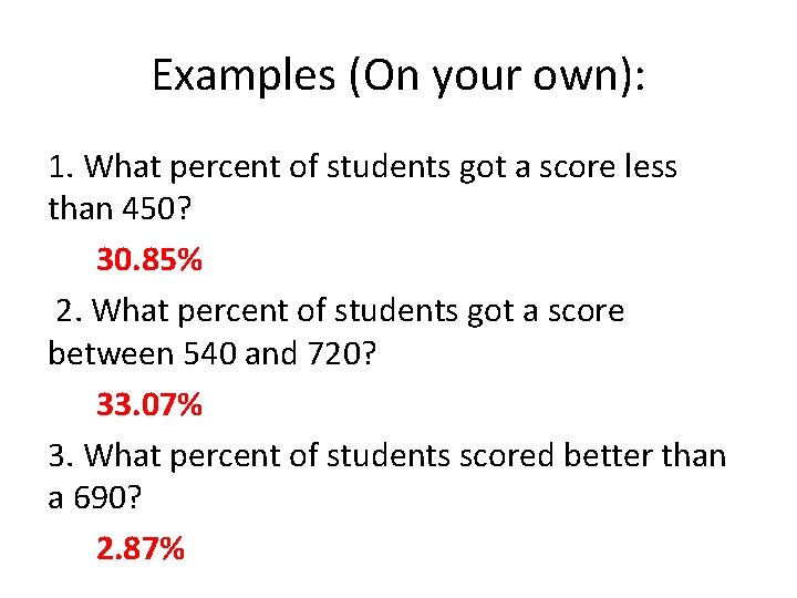
Examples (On your own): 1. What percent of students got a score less than 450? 30. 85% 2. What percent of students got a score between 540 and 720? 33. 07% 3. What percent of students scored better than a 690? 2. 87%

Classwork: Using Technology to Find Normal Percentages (Use the technology to do the examples on last slide for comparison)

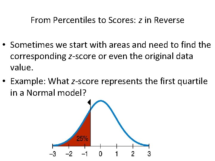
From Percentiles to Scores: z in Reverse • Sometimes we start with areas and need to find the corresponding z-score or even the original data value. • Example: What z-score represents the first quartile in a Normal model?

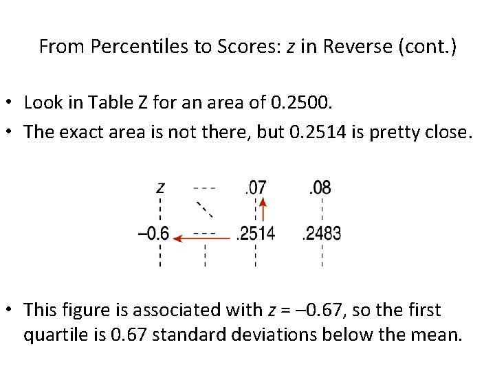
From Percentiles to Scores: z in Reverse (cont. ) • Look in Table Z for an area of 0. 2500. • The exact area is not there, but 0. 2514 is pretty close. • This figure is associated with z = – 0. 67, so the first quartile is 0. 67 standard deviations below the mean.

Technology: To find the z-score for a percentile: Go to 2 nd DIST. Use the function inv. Norm In the parentheses, put the percentile in decimal form. Examples: 1. Find the z-score at the 25 th percentile. -0. 67 2. Find the z-score at the 77 th percentile. 0. 74

Classwork: Flow chart between data, z scores, and percentiles. Normal Sheets A, B, and C

Are You Normal? How Can You Tell? • When you actually have your own data, you must check to see whether a Normal model is reasonable. • Looking at a histogram of the data is a good way.

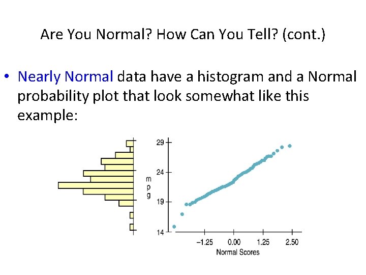
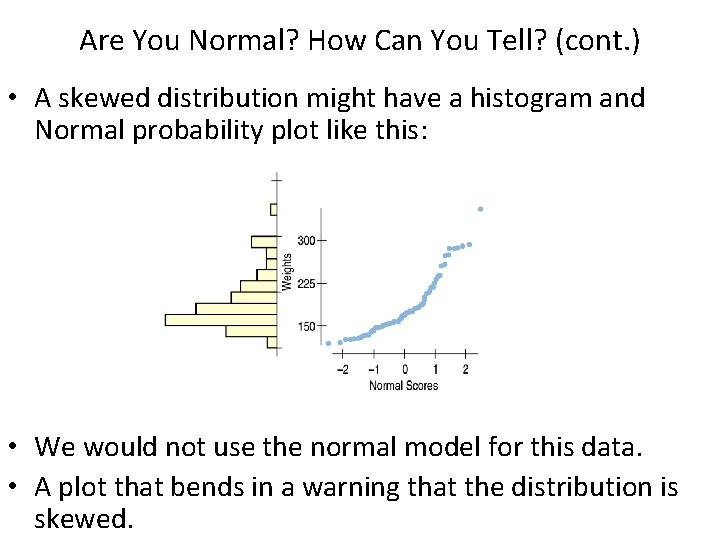
Are You Normal? How Can You Tell? (cont. ) • Another display that can help you decide whether a Normal model is appropriate is the Normal probability plot. • If the distribution is roughly Normal, the Normal probability plot approximates a diagonal straight line. • If the line is not straight, the distribution is not Normal.

Are You Normal? How Can You Tell? (cont. ) • Nearly Normal data have a histogram and a Normal probability plot that look somewhat like this example:

Are You Normal? How Can You Tell? (cont. ) • A skewed distribution might have a histogram and Normal probability plot like this: • We would not use the normal model for this data. • A plot that bends in a warning that the distribution is skewed.

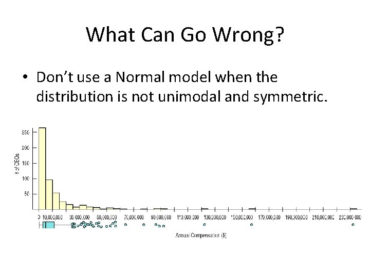
What Can Go Wrong? • Don’t use a Normal model when the distribution is not unimodal and symmetric.

What Can Go Wrong? (cont. ) • Don’t use the mean and standard deviation when outliers are present—the mean and standard deviation can both be distorted by outliers. • Don’t round off too soon. • Don’t round your results in the middle of a calculation. • Don’t worry about minor differences in results.

What have we learned? • The story data can tell may be easier to understand after shifting or rescaling the data. – Shifting data by adding or subtracting the same amount from each value affects measures of center and position but not measures of spread. – Rescaling data by multiplying or dividing every value by a constant changes all the summary statistics—center, position, and spread.

What have we learned? (cont. ) • We’ve learned the power of standardizing data. – Standardizing uses the SD as a ruler to measure distance from the mean (z-scores). – With z-scores, we can compare values from different distributions or values based on different units. – z-scores can identify unusual or surprising values among data.

What have we learned? (cont. ) • We’ve learned that the 68 -95 -99. 7 Rule can be a useful rule of thumb for understanding distributions: – For data that are unimodal and symmetric, about 68% fall within 1 SD of the mean, 95% fall within 2 SDs of the mean, and 99. 7% fall within 3 SDs of the mean.

What have we learned? (cont. ) • We see the importance of Thinking about whether a method will work: – Normality Assumption: We sometimes work with Normal tables (Table Z). These tables are based on the Normal model. – Data can’t be exactly Normal, so we check the Nearly Normal Condition by making a histogram (is it unimodal, symmetric and free of outliers? ) or a normal probability plot (is it straight enough? ).

Homework 1. Pg 134 – 136 Ex: 32 – 34, 37, 39, 41, 43, 48 2. Finish Reading Chapter 5 3. Complete Guided Reading Chapter 5 Test tomorrow