Chapter 7 An Introduction to Portfolio Management Questions

Chapter 7 - An Introduction to Portfolio Management Questions to be answered: l What do we mean by risk aversion and what evidence indicates that investors are generally risk averse? l What are the basic assumptions behind the Markowitz portfolio theory? l What is meant by risk and what are some of the alternative measures of risk used in investments? l How do you compute the expected rate of return for an individual risky asset or a portfolio of assets? l How do you compute the standard deviation of rates of return for an individual risky asset? l What is meant by the covariance between rates of return and how do you compute covariance?

Chapter 7 - An Introduction to Portfolio Management l l l l What is the relationship between covariance and correlation? What is the formula for the standard deviation for a portfolio of risky assets and how does it differ from the standard deviation of an individual risky asset? Given the formula for the standard deviation of a portfolio, how and why do you diversify a portfolio? What happens to the standard deviation of a portfolio when you change the correlation between the assets in the portfolio? What is the risk-return efficient frontier? Is it reasonable for alternative investors to select different portfolios from the portfolios on the efficient frontier? What determines which portfolio on the efficient frontier is selected by an individual investor?

Background Assumptions l l As an investor you want to maximize the returns for a given level of risk. Your portfolio includes all of your assets and liabilities The relationship between the returns for assets in the portfolio is important. A good portfolio is not simply a collection of individually good investments.

Risk Aversion l l Given a choice between two assets with equal rates of return, most investors will select the asset with the lower level of risk. Evidence That Investors are Risk Averse l l l Many investors purchase insurance for: Life, Automobile, Health, and Disability Income. The purchaser trades known costs for unknown risk of loss Yield on bonds increases with risk classifications from AAA to A…. Not all investors are risk averse l Risk preference may have to do with amount of money involved risking small amounts, but insuring large losses

Markowitz Portfolio Theory l l Quantifies risk Derives the expected rate of return for a portfolio of assets and an expected risk measure Shows that the variance of the rate of return is a meaningful measure of portfolio risk Derives the formula for computing the variance of a portfolio, showing how to effectively diversify a portfolio

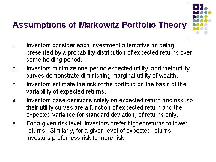
Assumptions of Markowitz Portfolio Theory 1. 2. 3. 4. 5. Investors consider each investment alternative as being presented by a probability distribution of expected returns over some holding period. Investors minimize one-period expected utility, and their utility curves demonstrate diminishing marginal utility of wealth. Investors estimate the risk of the portfolio on the basis of the variability of expected returns. Investors base decisions solely on expected return and risk, so their utility curves are a function of expected return and the expected variance (or standard deviation) of returns only. For a given risk level, investors prefer higher returns to lower returns. Similarly, for a given level of expected returns, investors prefer less risk to more risk.

Markowitz Portfolio Theory Using these five assumptions, a single asset or portfolio of assets is considered to be efficient if no other asset or portfolio of assets offers higher expected return with the same (or lower) risk, or lower risk with the same (or higher) expected return.

Alternative Measures of Risk l l l Variance or standard deviation of expected return Range of returns Returns below expectations l l Semivariance – a measure that only considers deviations below the mean These measures of risk implicitly assume that investors want to minimize the damage from returns less than some target rate

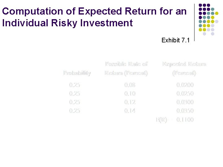
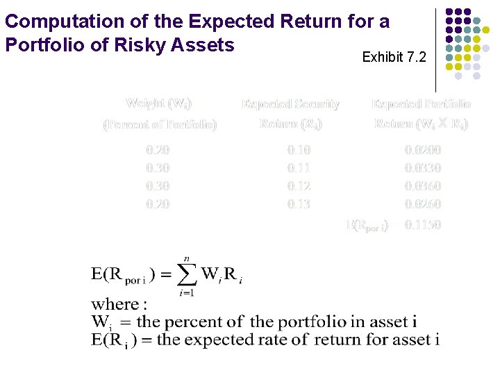
Expected Rates of Return l l For an individual asset - sum of the potential returns multiplied with the corresponding probability of the returns For a portfolio of assets - weighted average of the expected rates of return for the individual investments in the portfolio

Computation of Expected Return for an Individual Risky Investment Exhibit 7. 1

Computation of the Expected Return for a Portfolio of Risky Assets Exhibit 7. 2

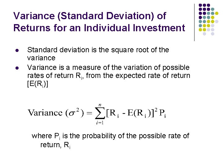
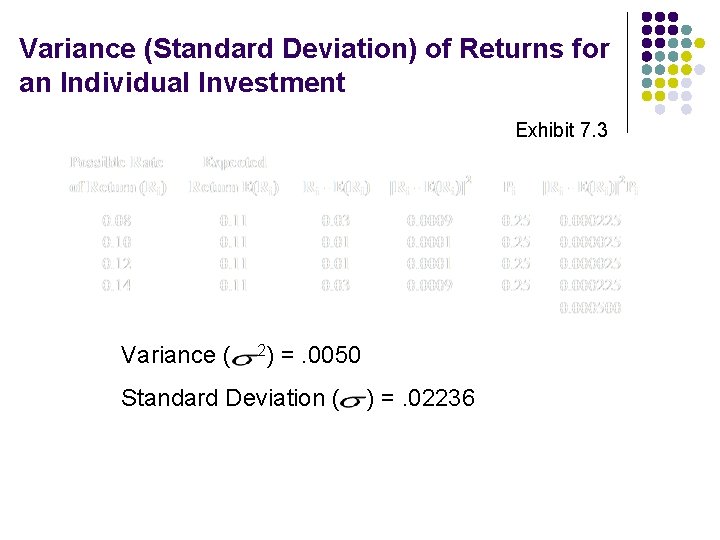
Variance (Standard Deviation) of Returns for an Individual Investment l l Standard deviation is the square root of the variance Variance is a measure of the variation of possible rates of return Ri, from the expected rate of return [E(Ri)] where Pi is the probability of the possible rate of return, Ri

Variance (Standard Deviation) of Returns for an Individual Investment Exhibit 7. 3 Variance ( 2) =. 0050 Standard Deviation ( ) =. 02236

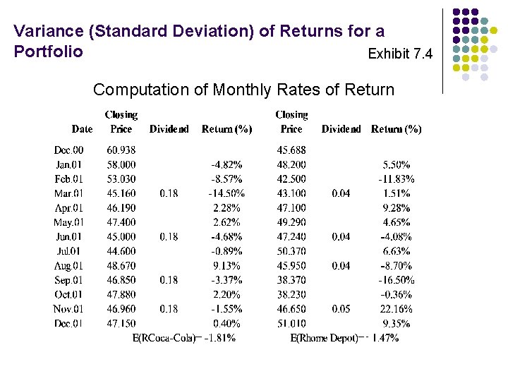
Variance (Standard Deviation) of Returns for a Portfolio Exhibit 7. 4 Computation of Monthly Rates of Return

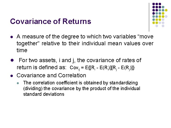
Covariance of Returns l A measure of the degree to which two variables “move together” relative to their individual mean values over time l For two assets, i and j, the covariance of rates of l return is defined as: Covij = E{[Ri - E(Ri)][Rj - E(Rj)]} Covariance and Correlation l The correlation coefficient is obtained by standardizing (dividing) the covariance by the product of the individual standard deviations

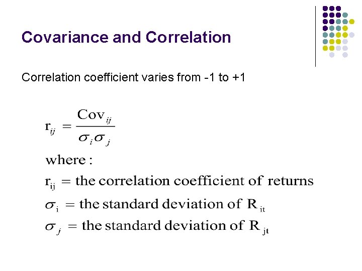
Covariance and Correlation coefficient varies from -1 to +1

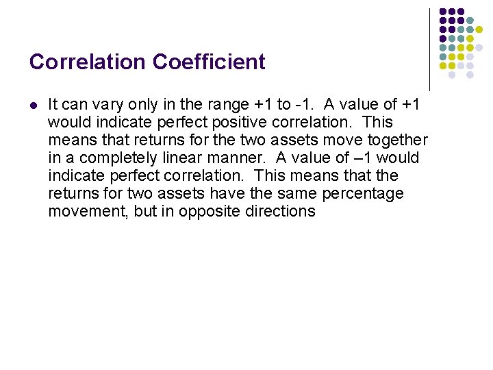
Correlation Coefficient l It can vary only in the range +1 to -1. A value of +1 would indicate perfect positive correlation. This means that returns for the two assets move together in a completely linear manner. A value of – 1 would indicate perfect correlation. This means that the returns for two assets have the same percentage movement, but in opposite directions

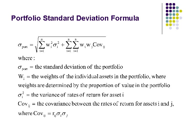
Portfolio Standard Deviation Formula

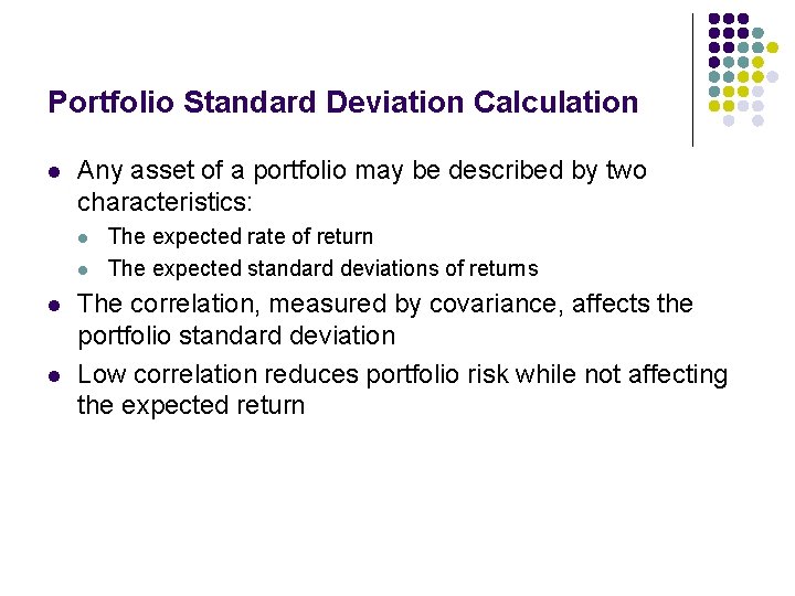
Portfolio Standard Deviation Calculation l Any asset of a portfolio may be described by two characteristics: l l The expected rate of return The expected standard deviations of returns The correlation, measured by covariance, affects the portfolio standard deviation Low correlation reduces portfolio risk while not affecting the expected return

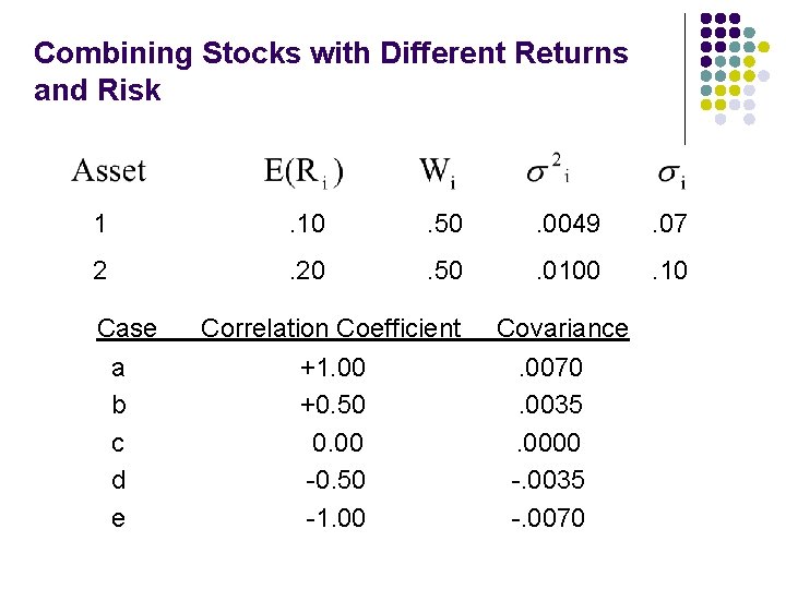
Combining Stocks with Different Returns and Risk 1 . 10 . 50 . 0049 . 07 2 . 20 . 50 . 0100 . 10 Case a b c d e Correlation Coefficient +1. 00 +0. 50 0. 00 -0. 50 -1. 00 Covariance. 0070. 0035. 0000 -. 0035 -. 0070

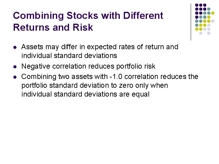
Combining Stocks with Different Returns and Risk l l l Assets may differ in expected rates of return and individual standard deviations Negative correlation reduces portfolio risk Combining two assets with -1. 0 correlation reduces the portfolio standard deviation to zero only when individual standard deviations are equal

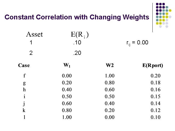
Constant Correlation with Changing Weights 1 . 10 2 . 20 r ij = 0. 00

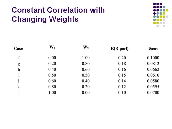
Constant Correlation with Changing Weights

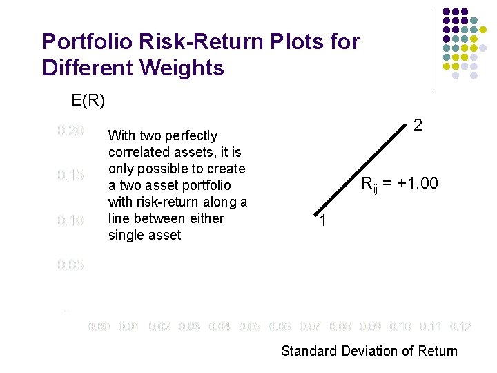
Portfolio Risk-Return Plots for Different Weights E(R) With two perfectly correlated assets, it is only possible to create a two asset portfolio with risk-return along a line between either single asset 2 Rij = +1. 00 1 Standard Deviation of Return

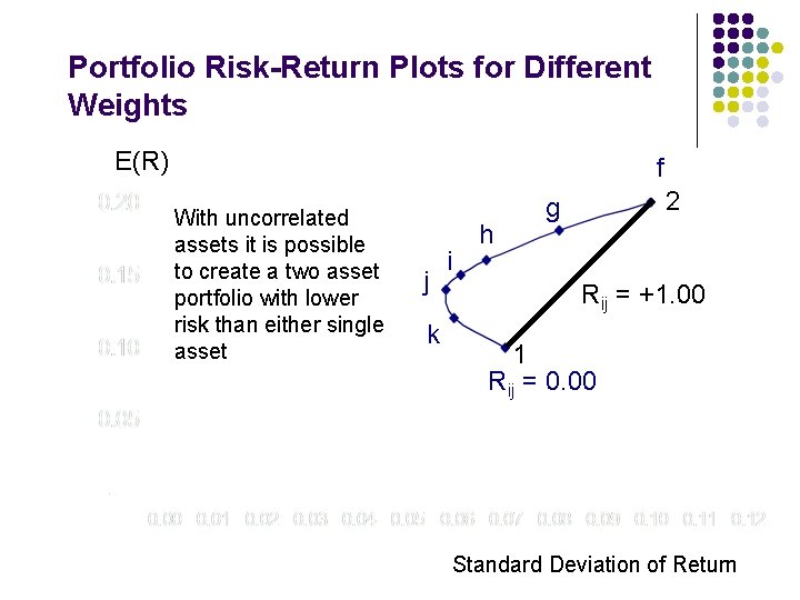
Portfolio Risk-Return Plots for Different Weights E(R) f With uncorrelated assets it is possible to create a two asset portfolio with lower risk than either single asset j k i h 2 g Rij = +1. 00 1 Rij = 0. 00 Standard Deviation of Return

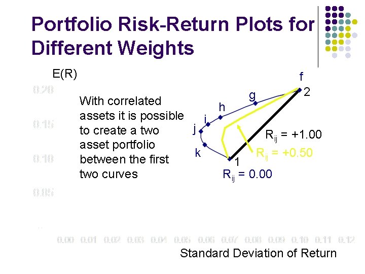
Portfolio Risk-Return Plots for Different Weights E(R) f g 2 With correlated h assets it is possible i j to create a two Rij = +1. 00 asset portfolio k Rij = +0. 50 between the first 1 Rij = 0. 00 two curves Standard Deviation of Return

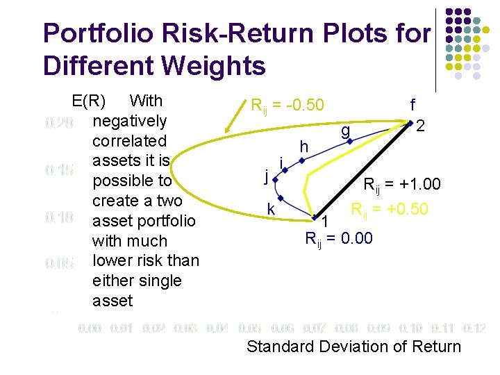
Portfolio Risk-Return Plots for Different Weights E(R) With negatively correlated assets it is possible to create a two asset portfolio with much lower risk than either single asset Rij = -0. 50 j k i h f 2 g Rij = +1. 00 Rij = +0. 50 1 Rij = 0. 00 Standard Deviation of Return

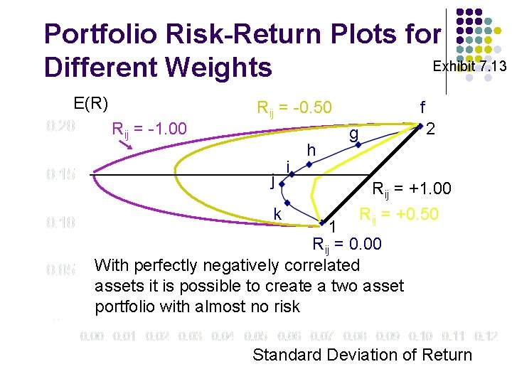
Portfolio Risk-Return Plots for Exhibit 7. 13 Different Weights E(R) Rij = -1. 00 Rij = -0. 50 j k i h f 2 g Rij = +1. 00 Rij = +0. 50 1 Rij = 0. 00 With perfectly negatively correlated assets it is possible to create a two asset portfolio with almost no risk Standard Deviation of Return

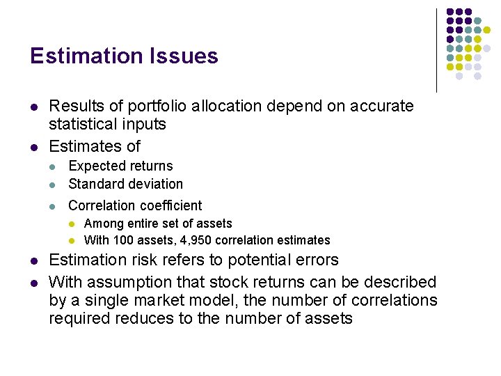
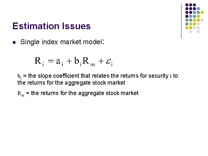
Estimation Issues l l Results of portfolio allocation depend on accurate statistical inputs Estimates of l Expected returns Standard deviation l Correlation coefficient l l l Among entire set of assets With 100 assets, 4, 950 correlation estimates Estimation risk refers to potential errors With assumption that stock returns can be described by a single market model, the number of correlations required reduces to the number of assets

Estimation Issues l Single index market model: bi = the slope coefficient that relates the returns for security i to the returns for the aggregate stock market Rm = the returns for the aggregate stock market

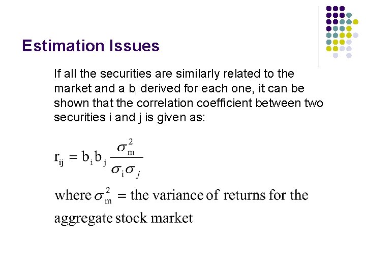
Estimation Issues If all the securities are similarly related to the market and a bi derived for each one, it can be shown that the correlation coefficient between two securities i and j is given as:

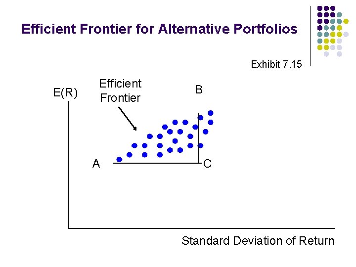
The Efficient Frontier l l The efficient frontier represents that set of portfolios with the maximum rate of return for every given level of risk, or the minimum risk for every level of return Frontier will be portfolios of investments rather than individual securities l Exceptions being the asset with the highest return and the asset with the lowest risk

Efficient Frontier for Alternative Portfolios Exhibit 7. 15 E(R) Efficient Frontier A B C Standard Deviation of Return

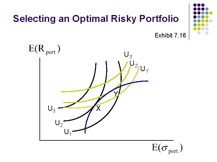
The Efficient Frontier and Investor Utility l l l An individual investor’s utility curve specifies the tradeoffs he is willing to make between expected return and risk The slope of the efficient frontier curve decreases steadily as you move upward These two interactions will determine the particular portfolio selected by an individual investor The optimal portfolio has the highest utility for a given investor It lies at the point of tangency between the efficient frontier and the utility curve with the highest possible utility

Selecting an Optimal Risky Portfolio Exhibit 7. 16 U 3’ U 2’ Y U 3 U 2 X U 1’