Risk and Return The objective to learn risk

Risk and Return

The objective to learn risk and return: n n The appropriate discount rate used in capital budgeting is the firm’s average cost of capital, that is, the weighted average of costs of debt and equity. While cost of debt is easy to estimate, the cost of equity is difficult to determine. The realized cost of equity does not always apply. ¨ We need to learn how equity holders determine their required rate of return when investing equity. ¨ The force of capital market would make the equity holders’ required rate of return equal to the true cost of equity. ¨

Risk and Return n Due to the return will be realized by the end of the period, so the investor will not know the return for sure, so the rate of return is only a random variable to the investor. The investor needs to estimate what will be the return.

The subjective way to describe random variable – Probability Distribution Outcomes Probability T-bill Corp. Bond Common Stock Serious Recession 0. 05 8% 12% -3% Mild recession 0. 20 8% 10% 6% stable 0. 50 8% 9% 11% Mild prosperity 0. 20 8% 8. 5% 14% Extreme prosperity 0. 05 8% 8% 19% Expected Return 8% 9. 2% 10. 3% Standard Deviation 0% 0. 84% 4. 39%

Expected Return Possible outcome probability Standard deviation

The difficulty in using the subjective Probability Distribution It is difficult to describe the probability distribution of an individual. n It is not certain that an individual’s probability distribution is in accordance with the probability distribution of investors of market as a whole, which is more relevant in determining cost of equity. n

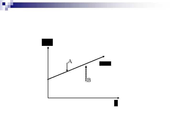
The objective way to describe random variable – historical data n We can measure risk and return employing historical returns. We basically believe that history will repeat itself. Expected Return Standard Deviation

The problems in using historical data in estimating risk and return Some of firms, start-up or private firms, may lack of stock trades information in estimating realized risk and return. n This historical estimation sometimes may not be representative for future expectations. n

Risk and return for two assets Ａ Expected return Standard deviation Investment ratio Expected return for the portfolio Standard deviation for the portfolio Ｂ

The definition of Covariance The covariance is to measure the comovement of two random variable. n When covariance is positive, then the two random variables tend to move into same direction. n When covariance is negative, then the two random variables tend to more to opposite directions. n

Risk and return for three assets Ａ Expected return Standard deviation Investment ratio Expected return for the portfolio Standard deviation for the portfolio Ｂ Ｃ

Risk and return for N assets Expected return Standard deviation

Risk Diversification n When number of assets increases, the majority of risk for the portfolio comes from the co-movement among assets. The distinctive risk comes from each asset becomes less important.

How diversification works Ａ Expected return Standard deviation Investment ratio 10% 4% 50% Ｂ 14% 6% 50%

Combining Stocks with Different Returns and Risk Assets may differ in expected rates of return and individual standard deviations n Negative or small positive correlations reduce portfolio risk n Combining two assets with -1. 0 correlation is able reduces the portfolio standard deviation to zero. n

Constant Correlation with Changing Weights 1 . 10 . 07 2 . 20 . 10 r ij = 1. 00

Portfolio Risk-Return Plots for Different Weights E(R) With two perfectly correlated assets, it is only possible to create a two asset portfolio with riskreturn along a line between either single asset 2 Rij = +1. 00 1 Standard Deviation of Return

Constant Correlation with Changing Weights 1 . 10 . 07 2 . 20 . 10 r ij = 0. 00

Portfolio Risk-Return Plots for Different Weights E(R) f g 2 With uncorrelated h assets it is possible i j to create a two Rij = +1. 00 asset portfolio with k lower risk than 1 Rij = 0. 00 either single asset Standard Deviation of Return

Portfolio Risk-Return Plots for Different Weights E(R) f g 2 With correlated h assets it is possible i j to create a two Rij = +1. 00 asset portfolio k Rij = +0. 50 between the first 1 Rij = 0. 00 two curves Standard Deviation of Return

Portfolio Risk-Return Plots for Different Weights E(R) With negatively correlated assets it is possible to create a two asset portfolio with much lower risk than either single asset Rij = -0. 50 j k i h f 2 g Rij = +1. 00 Rij = +0. 50 1 Rij = 0. 00 Standard Deviation of Return

Constant Correlation with Changing Weights 1 . 10 . 07 2 . 20 . 10 r ij = -1. 00

Portfolio Risk-Return Plots for Different Weights E(R) Rij = -1. 00 Rij = -0. 50 j k i h f 2 g Rij = +1. 00 Rij = +0. 50 1 Rij = 0. 00 With perfectly negatively correlated assets it is possible to create a two asset portfolio with almost no risk Standard Deviation of Return

A zero standard deviation for a two asset portfolio with correlation of -1 n When and , the investor is able to form a zero standard deviation (that is, zero risk) portfolio.

The Efficient Frontier The efficient frontier represents that set of portfolios, within all possibilities, with the highest rate of return for every given level of risk, or with the lowest risk for every given level of return n Efficient Frontier would be composed of portfolios rather than individual securities n ¨ Exceptions being the asset with the highest return and the asset with the lowest risk

Efficient Frontier for Alternative Portfolios E(R) Efficient Frontier A B C Standard Deviation of Return

The Efficient Frontier and an Investor’s Utility The optimal portfolio chosen has the highest utility for a given investor n The optimal portfolio lies at the point of tangency between the efficient frontier and the utility curve with the highest possible utility n

Selecting an Optimal Risky Portfolio U 3’ U 2’ Y U 3 U 2 X U 1’

Summary: n n n The efficient frontier derived from risky assets will be a curve, rather than a linear equation. Investors with different risk preferences will choose different points on efficient frontier to be their optimal choices. So the equilibrium will be on the whole efficient frontier. Problem: it is difficult to describe and apply a nonlinear relationship of risk and return. Solution: introduce a risk-free asset into the model…

Combining a Risk-Free Asset with a Risky Portfolio Since both the expected return and the standard deviation of return for such a portfolio are linear combinations for that risky portfolio and the risk free asset, a graph of possible portfolio returns and risks looks like a straight line between the two assets.

Risk-Free Asset An asset with zero standard deviation n Zero correlation with all other risky assets n Provides the risk-free rate of return (RFR) n Will lie on the vertical axis of a portfolio graph n

Risk-Free Asset Covariance between two sets of returns is Because the returns for the risk free asset are certain, Thus Ri = E(Ri), and Ri - E(Ri) = 0 Consequently, the covariance of the risk-free asset with any risky asset or portfolio will always equal zero. Similarly the correlation between any risky asset and the risk-free asset would be zero.

Combining a Risk-Free Asset with a Risky Portfolio Expected return the weighted average of the two returns This is a linear relationship

Combining a Risk-Free Asset with a Risky Portfolio Standard deviation Since we know that the variance of the risk-free asset is zero and the correlation between the risk-free asset and any risky asset i is zero we can adjust the formula

Capital Market Line (CML) M C RFR A B D

Portfolio Possibilities Combining the Risk-Free Asset and Risky Portfolios on the Efficient Frontier rr o B g n i nd Le RFR M o g n i w L M C

The Security Market Line (SML) The relevant risk measure for an individual risky asset is its covariance with the market portfolio (Covi, m) n This is shown as the risk measure n The return for the market portfolio should be consistent with its own risk, which is the covariance of the market with itself - or its variance: n

Graph of Security Market Line (SML) SML RFR

The Security Market Line (SML) The equation for the risk-return line is We then define as beta

Graph of SML with Normalized Systematic Risk SML Negative Beta RFR

Factors that influences the shape of SML Inflation risk premium (inflation expectation) n Investors’ attitude toward risk (risk aversion) n

Inflation risk premium

Investors’ attitude toward risk (risk aversion)

Capital Market equilibrium n The required rate of return: n The expected rate of return: n When expected return > required return ¨ Then n P 0 increases, expected return decreases When expected return < required return ¨ Then P 0 decreases, expected return increases