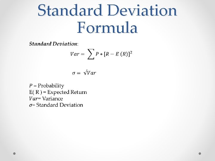
calculating Standard Deviation in Excel Standard Deviation Formula

calculating Standard Deviation in Excel

Standard Deviation Formula

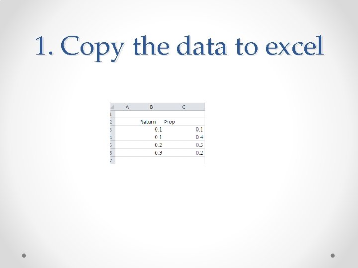
1. Copy the data to excel

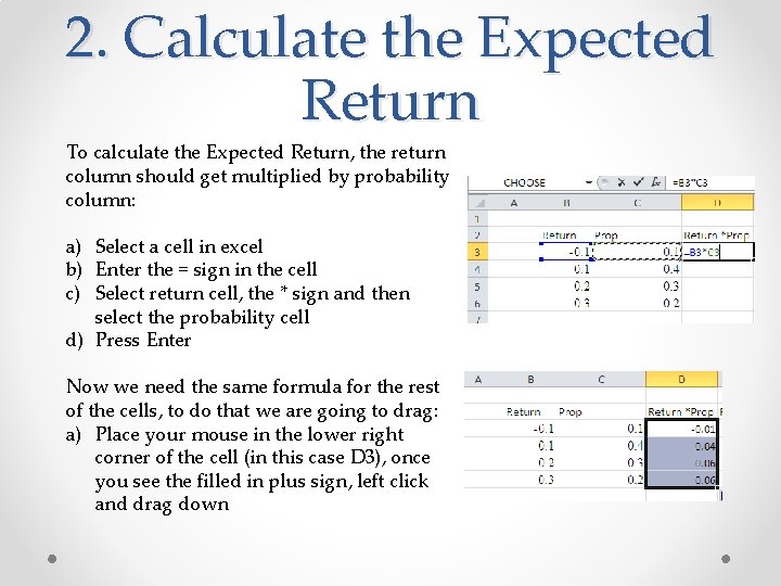
2. Calculate the Expected Return To calculate the Expected Return, the return column should get multiplied by probability column: a) Select a cell in excel b) Enter the = sign in the cell c) Select return cell, the * sign and then select the probability cell d) Press Enter Now we need the same formula for the rest of the cells, to do that we are going to drag: a) Place your mouse in the lower right corner of the cell (in this case D 3), once you see the filled in plus sign, left click and drag down

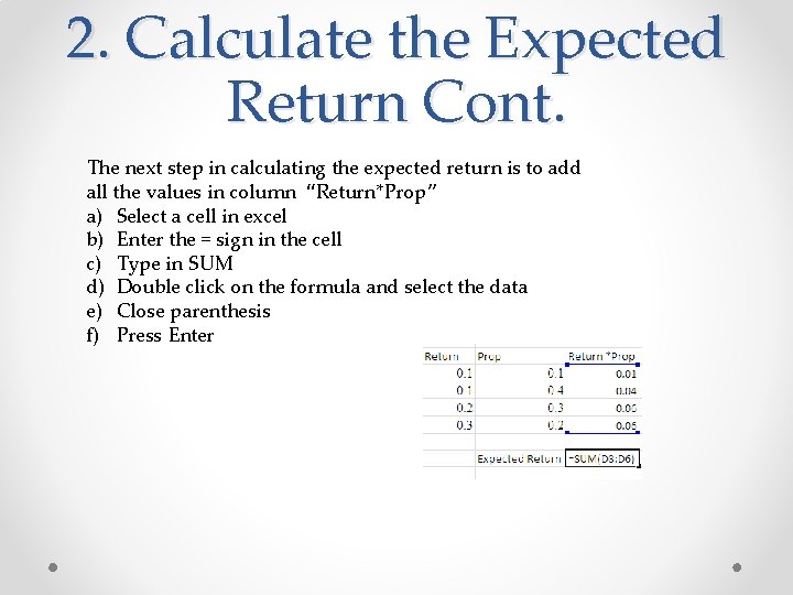
2. Calculate the Expected Return Cont. The next step in calculating the expected return is to add all the values in column “Return*Prop” a) Select a cell in excel b) Enter the = sign in the cell c) Type in SUM d) Double click on the formula and select the data e) Close parenthesis f) Press Enter

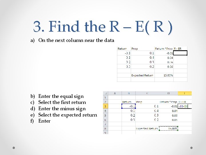
3. Find the R – E( R ) a) On the next column near the data b) c) d) e) f) Enter the equal sign Select the first return Enter the minus sign Select the expected return Enter

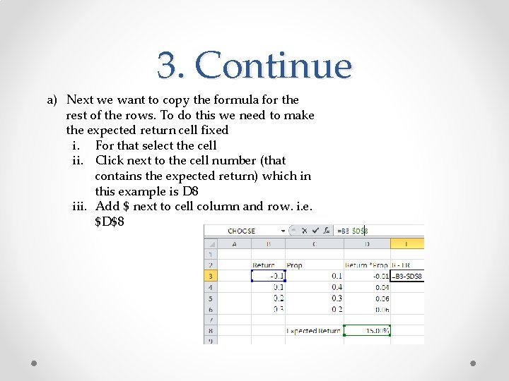
3. Continue a) Next we want to copy the formula for the rest of the rows. To do this we need to make the expected return cell fixed i. For that select the cell ii. Click next to the cell number (that contains the expected return) which in this example is D 8 iii. Add $ next to cell column and row. i. e. $D$8

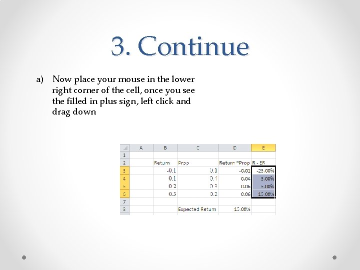
3. Continue a) Now place your mouse in the lower right corner of the cell, once you see the filled in plus sign, left click and drag down

4. [R – E( R )]^2 a) Go to the next column on the first row b) Enter the equal sign c) Select the R - ER cell, in this example E 3 d) Then Shift + 6 ( to add ^ sign) e) The number 2 f) Enter

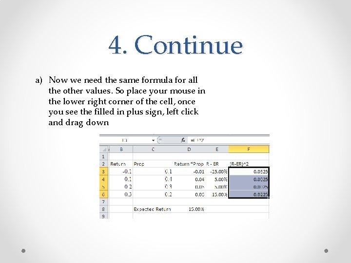
4. Continue a) Now we need the same formula for all the other values. So place your mouse in the lower right corner of the cell, once you see the filled in plus sign, left click and drag down

5. P * [R – E( R )]^2 a) Select a cell in excel b) Enter the = sign in the cell c) Select probability cell, the * sign and then select the [R – E( R )]^2 cell d) Press Enter

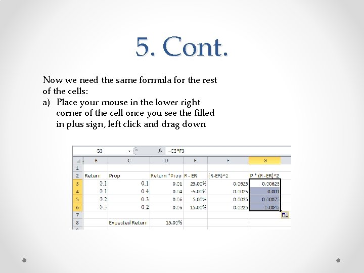
5. Cont. Now we need the same formula for the rest of the cells: a) Place your mouse in the lower right corner of the cell once you see the filled in plus sign, left click and drag down

6. Sum P*[R – E( R )]^2 a) b) c) d) e) f) Select a cell Enter the equal sign Enter the word SUM Double click on the formula Select the data Enter

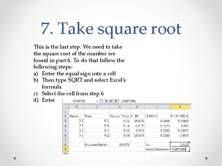
7. Take square root This is the last step. We need to take the square root of the number we found in part 6. To do that follow the following steps: a) Enter the equal sign into a cell b) Then type SQRT and select Excel's formula c) Select the cell from step 6 d) Enter