Chapter 4 Mathematical Expectation 4 1 Chapter Outline

Chapter 4 Mathematical Expectation 4 -1

Chapter Outline 4. 1 Mean of a Random Variable 4. 2 Variance of Random Variables 4. 3 Means and Variances of Linear Combinations of Random Variables 3 -2

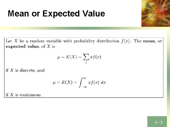
Mean or Expected Value 4 -3

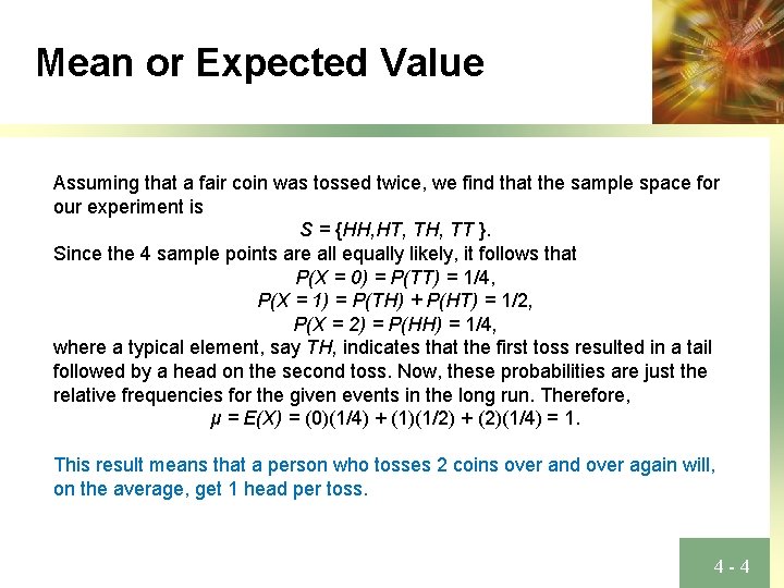
Mean or Expected Value Assuming that a fair coin was tossed twice, we find that the sample space for our experiment is S = {HH, HT, TH, TT }. Since the 4 sample points are all equally likely, it follows that P(X = 0) = P(TT) = 1/4, P(X = 1) = P(TH) + P(HT) = 1/2, P(X = 2) = P(HH) = 1/4, where a typical element, say TH, indicates that the first toss resulted in a tail followed by a head on the second toss. Now, these probabilities are just the relative frequencies for the given events in the long run. Therefore, μ = E(X) = (0)(1/4) + (1)(1/2) + (2)(1/4) = 1. This result means that a person who tosses 2 coins over and over again will, on the average, get 1 head per toss. 4 -4

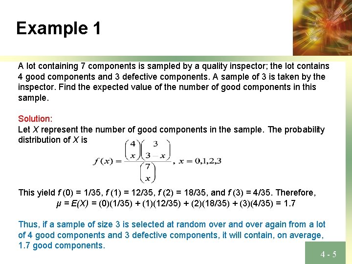
Example 1 A lot containing 7 components is sampled by a quality inspector; the lot contains 4 good components and 3 defective components. A sample of 3 is taken by the inspector. Find the expected value of the number of good components in this sample. Solution: Let X represent the number of good components in the sample. The probability distribution of X is This yield f (0) = 1/35, f (1) = 12/35, f (2) = 18/35, and f (3) = 4/35. Therefore, μ = E(X) = (0)(1/35) + (1)(12/35) + (2)(18/35) + (3)(4/35) = 1. 7 Thus, if a sample of size 3 is selected at random over and over again from a lot of 4 good components and 3 defective components, it will contain, on average, 1. 7 good components. 4 -5

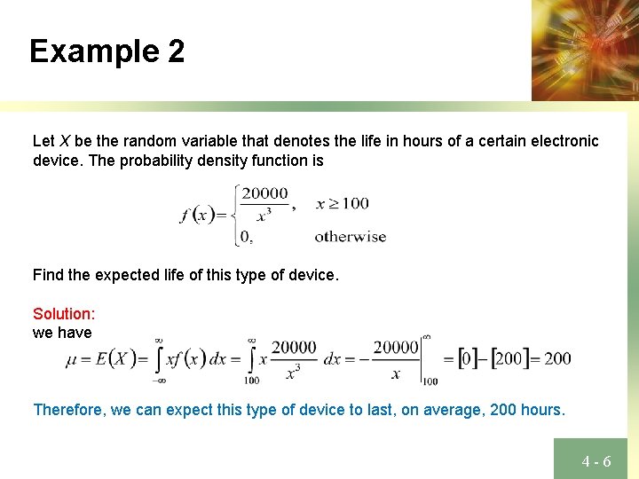
Example 2 Let X be the random variable that denotes the life in hours of a certain electronic device. The probability density function is Find the expected life of this type of device. Solution: we have Therefore, we can expect this type of device to last, on average, 200 hours. 4 -6

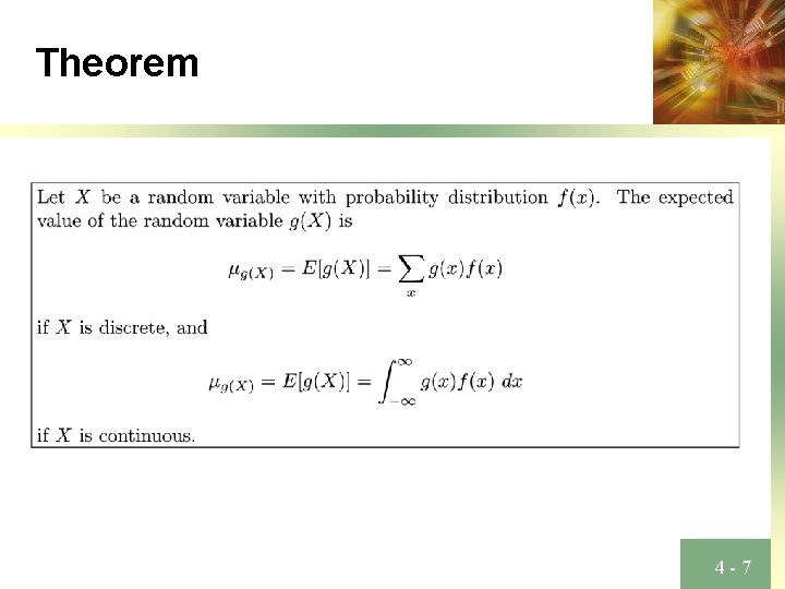
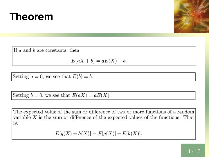
Theorem 4 -7

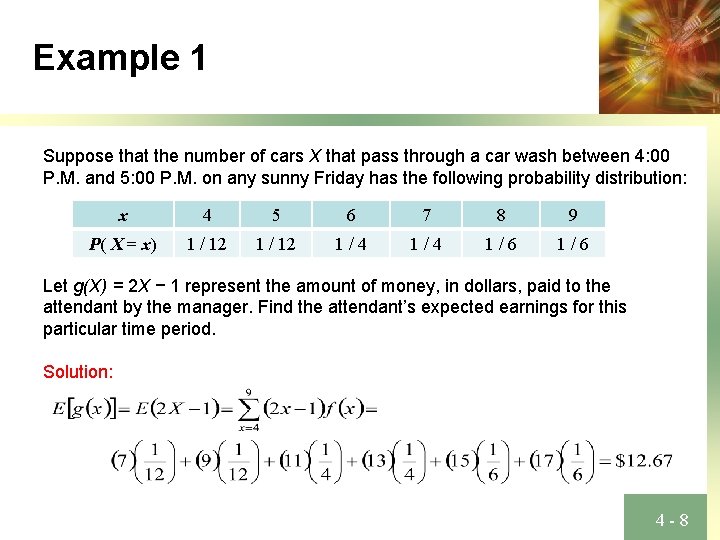
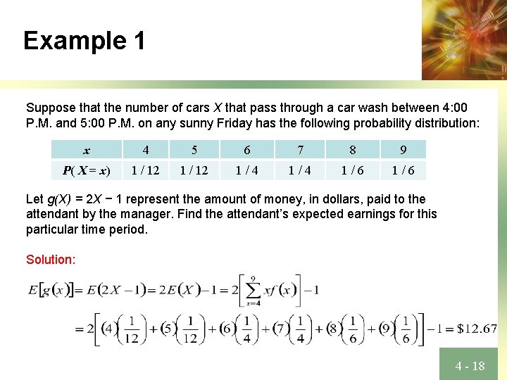
Example 1 Suppose that the number of cars X that pass through a car wash between 4: 00 P. M. and 5: 00 P. M. on any sunny Friday has the following probability distribution: x 4 5 6 7 8 9 P( X = x) 1 / 12 1/4 1/6 Let g(X) = 2 X − 1 represent the amount of money, in dollars, paid to the attendant by the manager. Find the attendant’s expected earnings for this particular time period. Solution: 4 -8

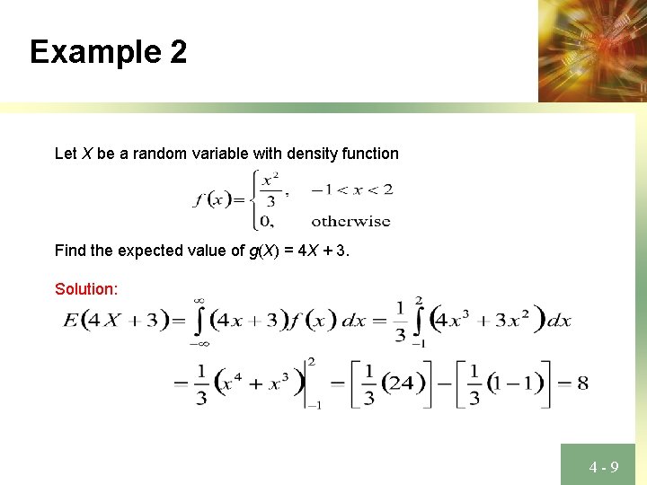
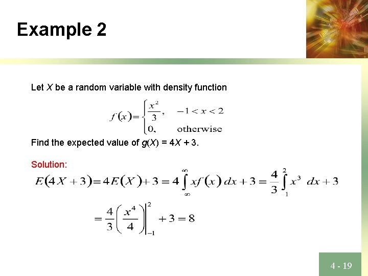
Example 2 Let X be a random variable with density function Find the expected value of g(X) = 4 X + 3. Solution: 4 -9

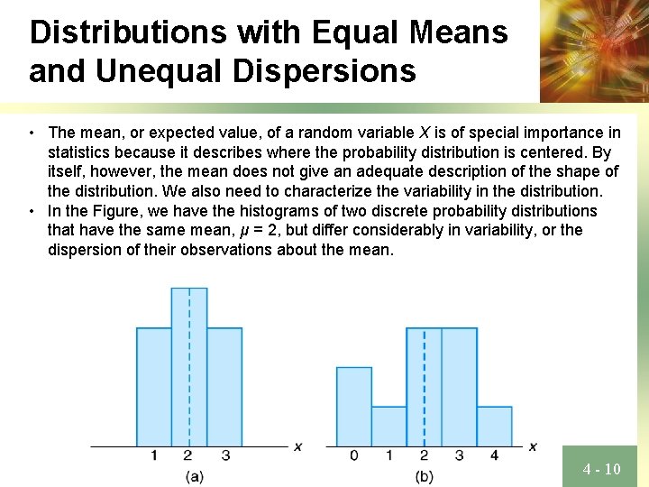
Distributions with Equal Means and Unequal Dispersions • The mean, or expected value, of a random variable X is of special importance in statistics because it describes where the probability distribution is centered. By itself, however, the mean does not give an adequate description of the shape of the distribution. We also need to characterize the variability in the distribution. • In the Figure, we have the histograms of two discrete probability distributions that have the same mean, μ = 2, but differ considerably in variability, or the dispersion of their observations about the mean. 4 - 10

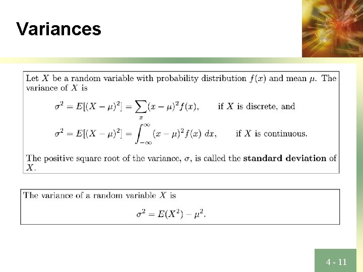
Variances 4 - 11

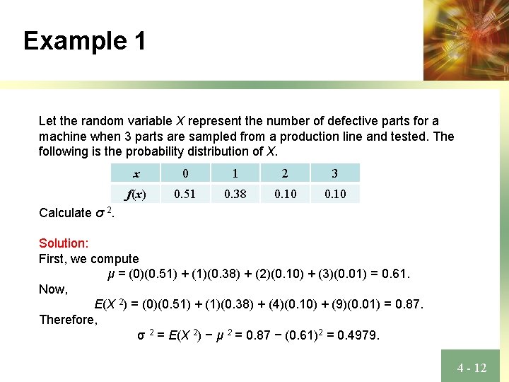
Example 1 Let the random variable X represent the number of defective parts for a machine when 3 parts are sampled from a production line and tested. The following is the probability distribution of X. x 0 1 2 3 f(x) 0. 51 0. 38 0. 10 Calculate σ 2. Solution: First, we compute μ = (0)(0. 51) + (1)(0. 38) + (2)(0. 10) + (3)(0. 01) = 0. 61. Now, E(X 2) = (0)(0. 51) + (1)(0. 38) + (4)(0. 10) + (9)(0. 01) = 0. 87. Therefore, σ 2 = E(X 2) − μ 2 = 0. 87 − (0. 61)2 = 0. 4979. 4 - 12

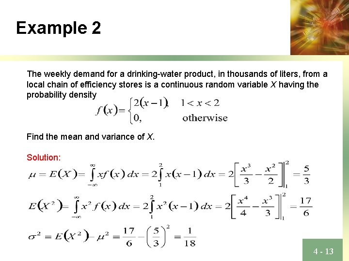
Example 2 The weekly demand for a drinking-water product, in thousands of liters, from a local chain of efficiency stores is a continuous random variable X having the probability density Find the mean and variance of X. Solution: 4 - 13

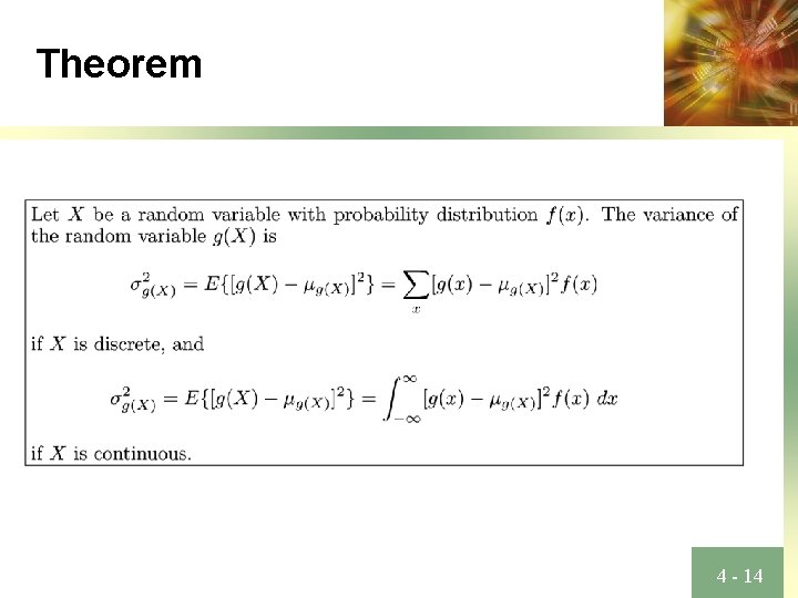
Theorem 4 - 14

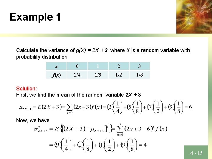
Example 1 Calculate the variance of g(X) = 2 X + 3, where X is a random variable with probability distribution x 0 1 2 3 f(x) 1/4 1/8 1/2 1/8 Solution: First, we find the mean of the random variable 2 X + 3 Now, we have 4 - 15

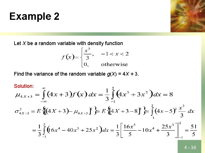
Example 2 Let X be a random variable with density function Find the variance of the random variable g(X) = 4 X + 3. Solution: 4 - 16

Theorem 4 - 17

Example 1 Suppose that the number of cars X that pass through a car wash between 4: 00 P. M. and 5: 00 P. M. on any sunny Friday has the following probability distribution: x 4 5 6 7 8 9 P( X = x) 1 / 12 1/4 1/6 Let g(X) = 2 X − 1 represent the amount of money, in dollars, paid to the attendant by the manager. Find the attendant’s expected earnings for this particular time period. Solution: 4 - 18

Example 2 Let X be a random variable with density function Find the expected value of g(X) = 4 X + 3. Solution: 4 - 19

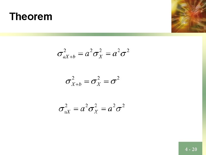
Theorem 4 - 20

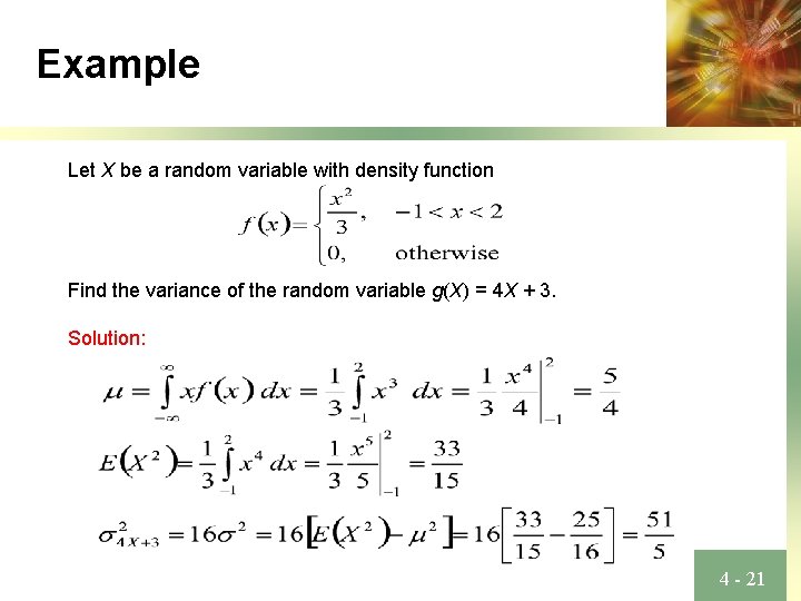
Example Let X be a random variable with density function Find the variance of the random variable g(X) = 4 X + 3. Solution: 4 - 21