Mathematical Expectation Spiegel et al 2000 Chapter 3

Mathematical Expectation Spiegel et al (2000) - Chapter 3 Examples by Mansoor Al-Harthy Maria Sanchez Sara Russell DP Kar Alex Lombardia Presented by Professor Carol Dahl

3 -2 Introduction Green Power Co. investment solar insolation (X) wind speed (W) Electricity hybrid (X, W) uncertainty characterize discrete random variable (X) probability function p(x) continuous random variable (W) probability density function f(w)

3 -3 Mathematical Expectation Expected Value Functions of Random Variables Some Theorems on Expectation The Variance and Standard Deviation Some Theorems on Variance Standardized Random Variables Moments Variances and Covariance for Joint Distributions Correlation Coefficient

3 -4 Mathematical Expectation Conditional Expectation & Variance Chebyshev's Inequality Law of Large Numbers Other Measures of Central Tendency Percentiles Other Measures of Dispersion Skewness and Kurtosis

3 -5 Random Variables value with a probability attached value never predicted with certainty not deterministic probabilistic

3 -6 Solar Insolation (m/s)

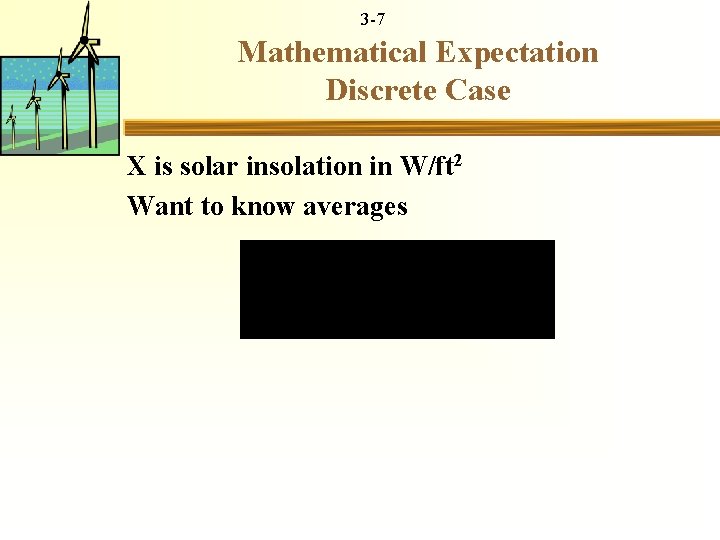
3 -7 Mathematical Expectation Discrete Case X is solar insolation in W/ft 2 Want to know averages

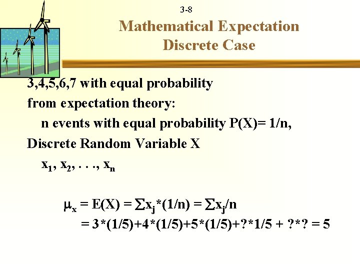
3 -8 Mathematical Expectation Discrete Case 3, 4, 5, 6, 7 with equal probability from expectation theory: n events with equal probability P(X)= 1/n, Discrete Random Variable X x 1, x 2, . . . , xn x = E(X) = xj*(1/n) = xj/n = 3*(1/5)+4*(1/5)+5*(1/5)+? *1/5 + ? *? = 5

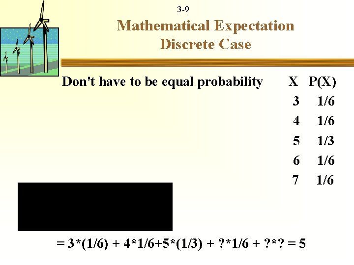
3 -9 Mathematical Expectation Discrete Case Don't have to be equal probability X P(X) 3 1/6 4 1/6 5 1/3 6 1/6 7 1/6 = 3*(1/6) + 4*1/6+5*(1/3) + ? *1/6 + ? *? = 5

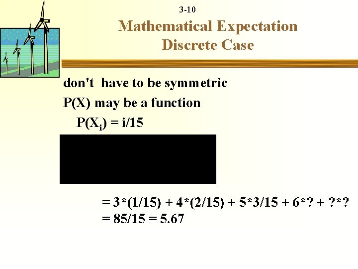
3 -10 Mathematical Expectation Discrete Case don't have to be symmetric P(X) may be a function P(Xi) = i/15 = 3*(1/15) + 4*(2/15) + 5*3/15 + 6*? + ? *? = 85/15 = 5. 67

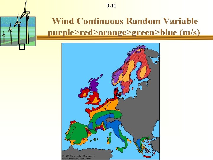
3 -11 Wind Continuous Random Variable purple>red>orange>green>blue (m/s) �

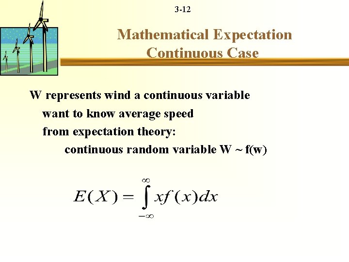
3 -12 Mathematical Expectation Continuous Case W represents wind a continuous variable want to know average speed from expectation theory: continuous random variable W ~ f(w)

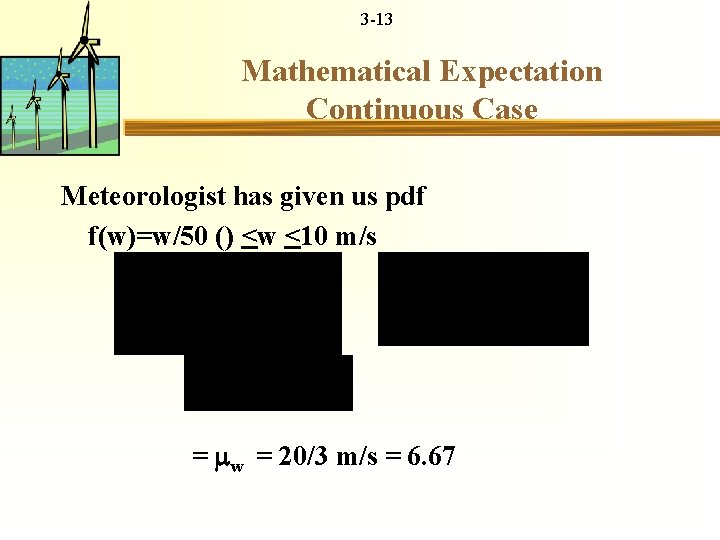
3 -13 Mathematical Expectation Continuous Case Meteorologist has given us pdf f(w)=w/50 () <w <10 m/s = w = 20/3 m/s = 6. 67

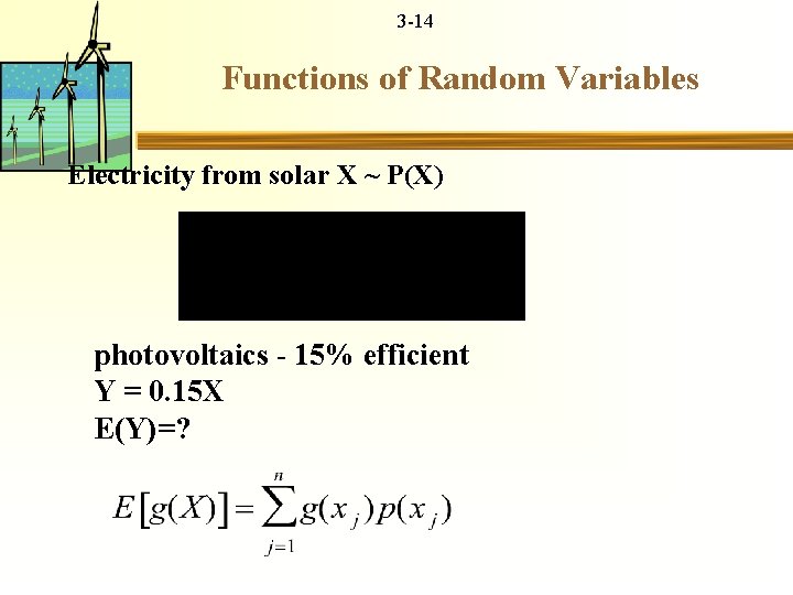
3 -14 Functions of Random Variables Electricity from solar X ~ P(X) photovoltaics - 15% efficient Y = 0. 15 X E(Y)=?

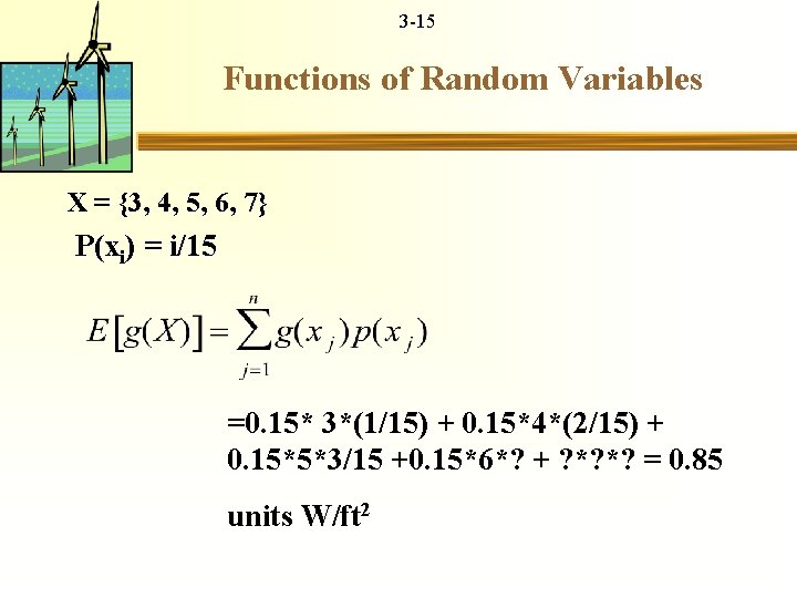
3 -15 Functions of Random Variables X = {3, 4, 5, 6, 7} P(xi) = i/15 =0. 15* 3*(1/15) + 0. 15*4*(2/15) + 0. 15*5*3/15 +0. 15*6*? + ? *? *? = 0. 85 units W/ft 2

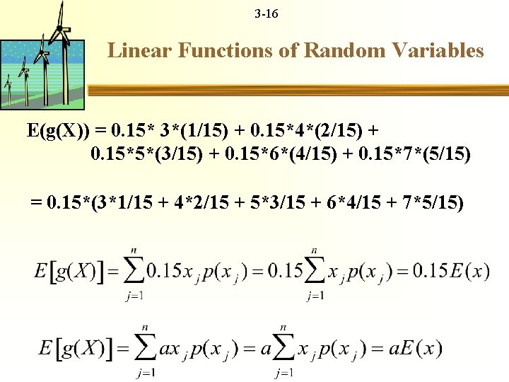
3 -16 Linear Functions of Random Variables E(g(X)) = 0. 15* 3*(1/15) + 0. 15*4*(2/15) + 0. 15*5*(3/15) + 0. 15*6*(4/15) + 0. 15*7*(5/15) = 0. 15*(3*1/15 + 4*2/15 + 5*3/15 + 6*4/15 + 7*5/15)

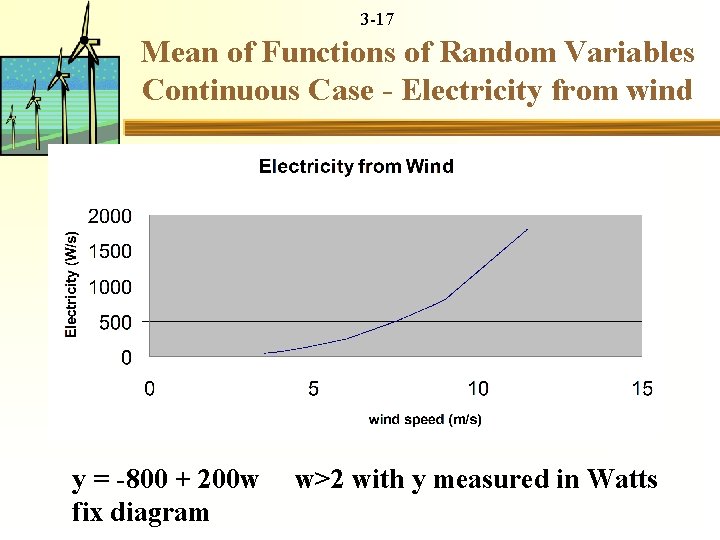
3 -17 Mean of Functions of Random Variables Continuous Case - Electricity from wind y = -800 + 200 w w>2 with y measured in Watts fix diagram

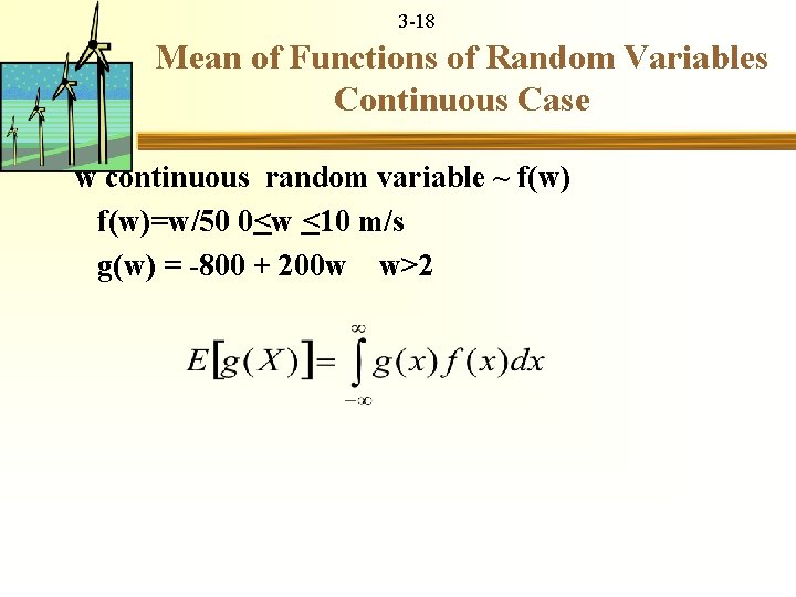
3 -18 Mean of Functions of Random Variables Continuous Case w continuous random variable ~ f(w)=w/50 0<w <10 m/s g(w) = -800 + 200 w w>2

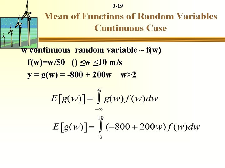
3 -19 Mean of Functions of Random Variables Continuous Case w continuous random variable ~ f(w)=w/50 () <w <10 m/s y = g(w) = -800 + 200 w w>2

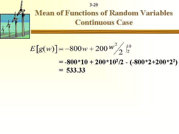
3 -20 Mean of Functions of Random Variables Continuous Case = -800*10 + 200*102/2 - (-800*2+200*22) = 533. 33

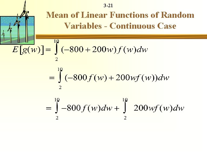
3 -21 Mean of Linear Functions of Random Variables - Continuous Case

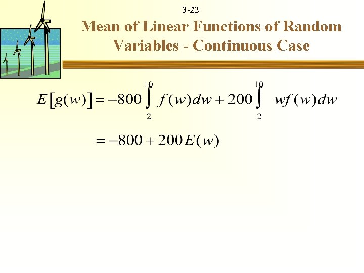
3 -22 Mean of Linear Functions of Random Variables - Continuous Case

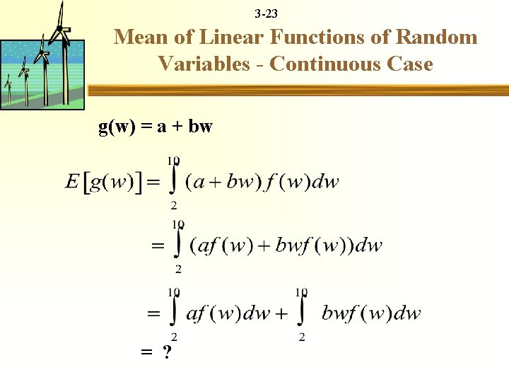
3 -23 Mean of Linear Functions of Random Variables - Continuous Case g(w) = a + bw = ?

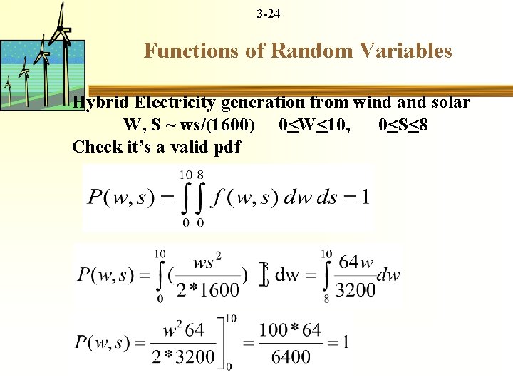
3 -24 Functions of Random Variables Hybrid Electricity generation from wind and solar W, S ~ ws/(1600) 0<W<10, 0<S<8 Check it’s a valid pdf

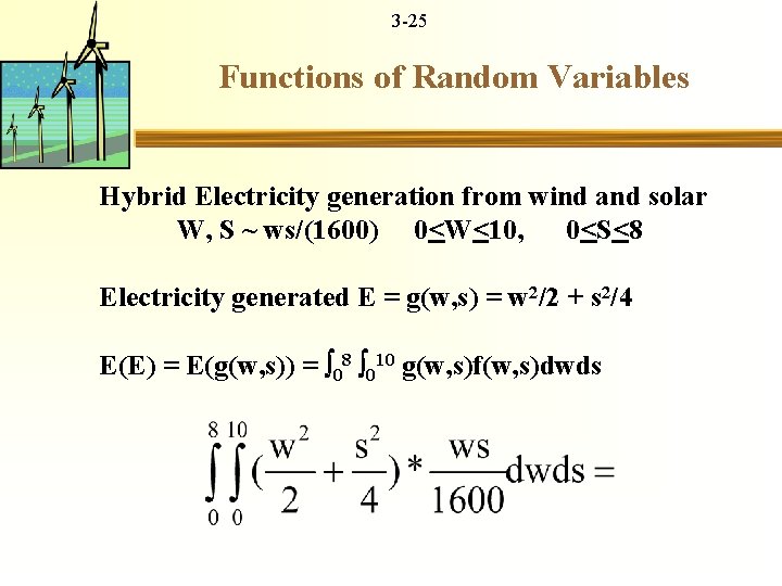
3 -25 Functions of Random Variables Hybrid Electricity generation from wind and solar W, S ~ ws/(1600) 0<W<10, 0<S<8 Electricity generated E = g(w, s) = w 2/2 + s 2/4 E(E) = E(g(w, s)) = 08 010 g(w, s)f(w, s)dwds

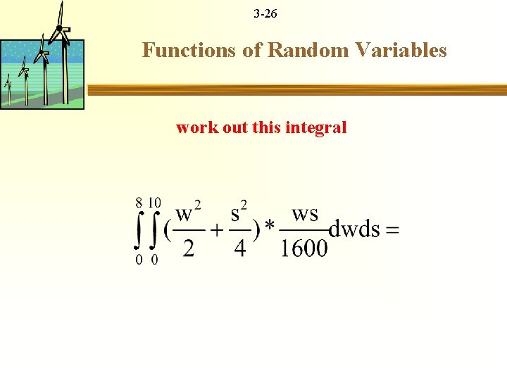
3 -26 Functions of Random Variables work out this integral

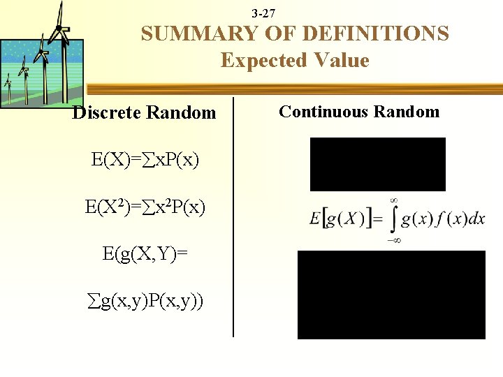
3 -27 SUMMARY OF DEFINITIONS Expected Value Discrete Random Continuous Random E(X)= x. P(x) E(X 2)= x 2 P(x) E(g(X, Y)= g(x, y)P(x, y))

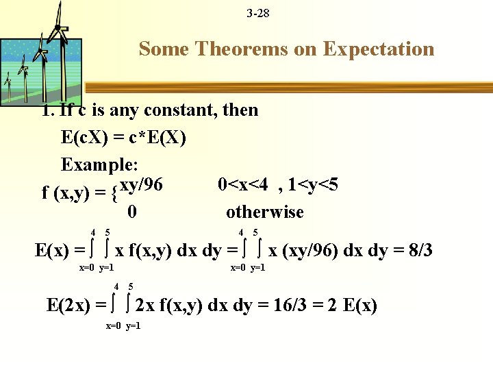
3 -28 Some Theorems on Expectation 1. If c is any constant, then E(c. X) = c*E(X) Example: f (x, y) = { xy/96 0 4 5 0<x<4 , 1<y<5 otherwise 4 5 E(x) = ∫ ∫ x f(x, y) dx dy = ∫ ∫ x (xy/96) dx dy = 8/3 x=0 y=1 4 5 E(2 x) = ∫ ∫ 2 x f(x, y) dx dy = 16/3 = 2 E(x) x=0 y=1

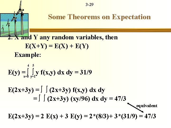
3 -29 Some Theorems on Expectation 2. X and Y any random variables, then E(X+Y) = E(X) + E(Y) Example: 4 5 E(y) = ∫ ∫ y f(x, y) dx dy = 31/9 x=0 y=1 E(2 x+3 y) = ∫ ∫ (2 x+3 y) f(x, y) dx dy = ∫ ∫ (2 x+3 y) (xy/96) dx dy = 47/3 equivalent E(2 x+3 y) = 2 E(x) + 3 E(y) = 2*(8/3)+ 3*(31/9) = 47/3

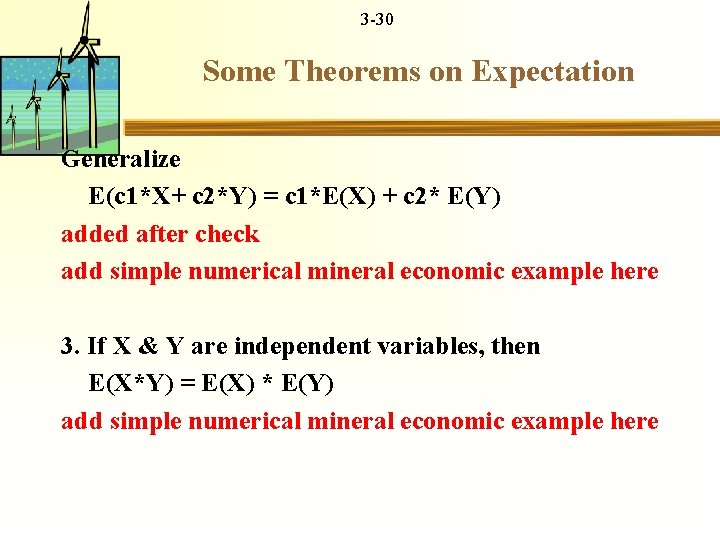
3 -30 Some Theorems on Expectation Generalize E(c 1*X+ c 2*Y) = c 1*E(X) + c 2* E(Y) added after check add simple numerical mineral economic example here 3. If X & Y are independent variables, then E(X*Y) = E(X) * E(Y) add simple numerical mineral economic example here

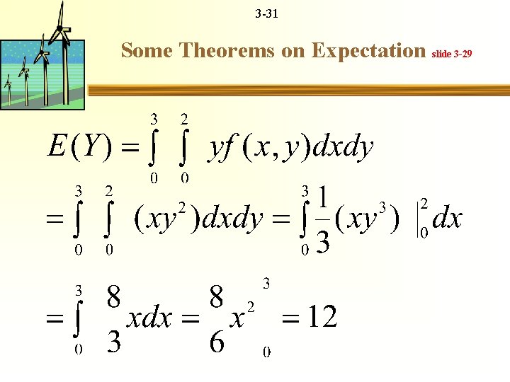
3 -31 Some Theorems on Expectation slide 3 -29

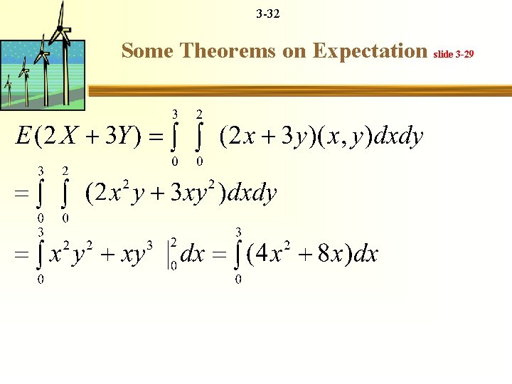
3 -32 Some Theorems on Expectation slide 3 -29

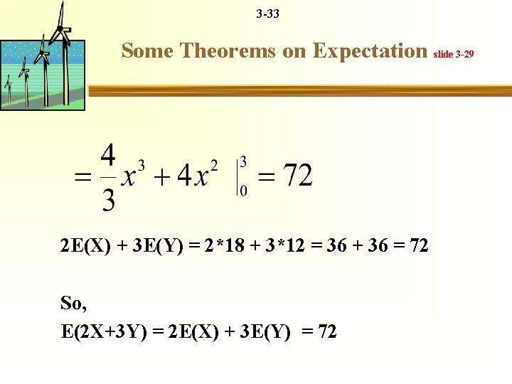
3 -33 Some Theorems on Expectation slide 3 -29 2 E(X) + 3 E(Y) = 2*18 + 3*12 = 36 + 36 = 72 So, E(2 X+3 Y) = 2 E(X) + 3 E(Y) = 72

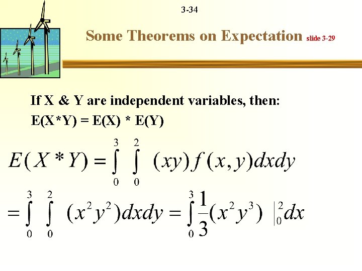
3 -34 Some Theorems on Expectation slide 3 -29 If X & Y are independent variables, then: E(X*Y) = E(X) * E(Y)

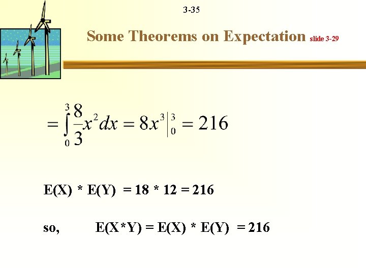
3 -35 Some Theorems on Expectation slide 3 -29 E(X) * E(Y) = 18 * 12 = 216 so, E(X*Y) = E(X) * E(Y) = 216

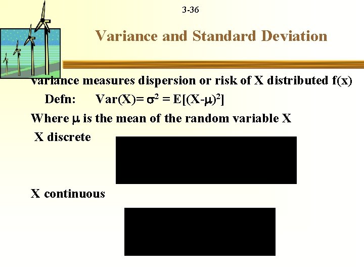
3 -36 Variance and Standard Deviation variance measures dispersion or risk of X distributed f(x) Defn: Var(X)= 2 = E[(X- )2] Where is the mean of the random variable X X discrete X continuous

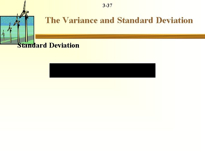
3 -37 The Variance and Standard Deviation

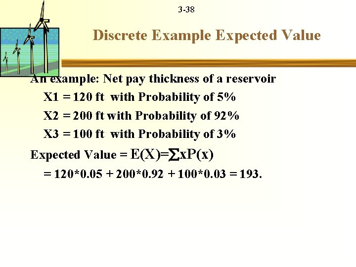
3 -38 Discrete Example Expected Value An example: Net pay thickness of a reservoir X 1 = 120 ft with Probability of 5% X 2 = 200 ft with Probability of 92% X 3 = 100 ft with Probability of 3% Expected Value = E(X)= x. P(x) = 120*0. 05 + 200*0. 92 + 100*0. 03 = 193.

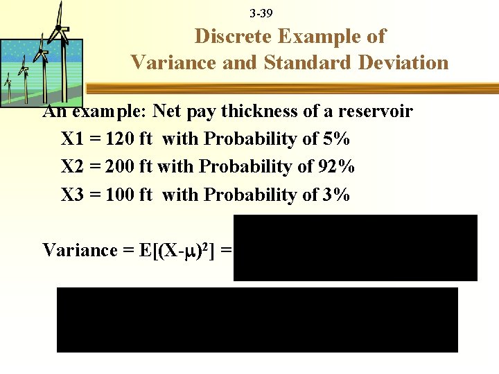
3 -39 Discrete Example of Variance and Standard Deviation An example: Net pay thickness of a reservoir X 1 = 120 ft with Probability of 5% X 2 = 200 ft with Probability of 92% X 3 = 100 ft with Probability of 3% Variance = E[(X- )2] =

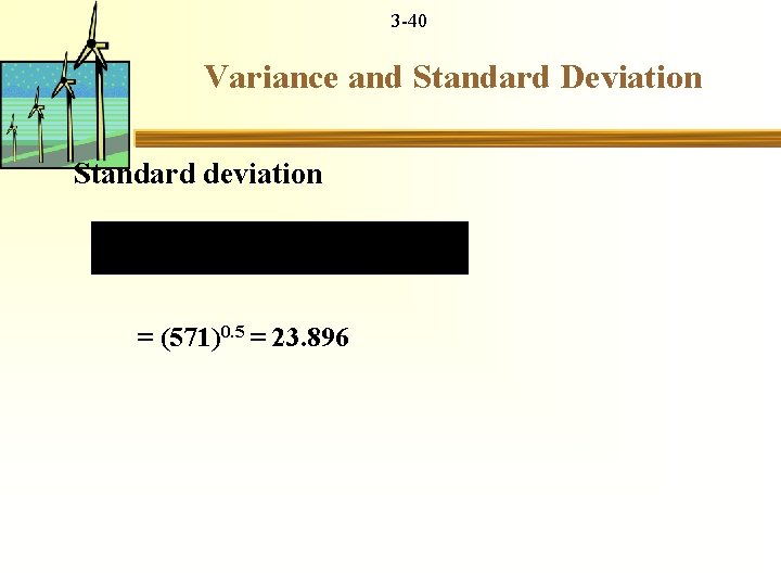
3 -40 Variance and Standard Deviation Standard deviation = (571)0. 5 = 23. 896

3 -41 Continuous Example Variance and Standard Deviation add continuous mineral econ example of mean and variance

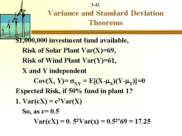
3 -42 Variance and Standard Deviation Theorems $1, 000 investment fund available, Risk of Solar Plant Var(X)=69, Risk of Wind Plant Var(Y)=61, X and Y independent Cov(X, Y)= XY = E[(X- X)(Y- Y)]=0 Expected Risk, if 50% fund in plant 1? 1. Var(c. X) = c 2 Var(X) So, as c= 0. 5 Var(c. X) = 0. 52 Var(x) = 0. 52*69 = 17. 25

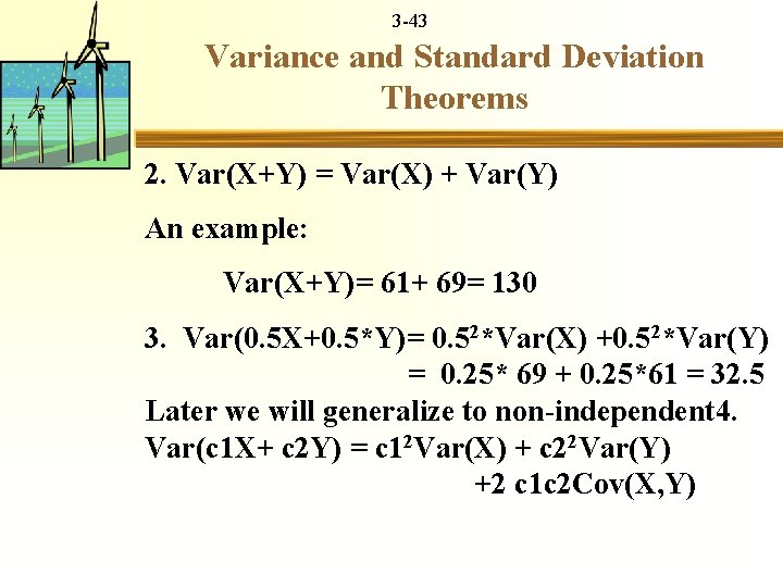
3 -43 Variance and Standard Deviation Theorems 2. Var(X+Y) = Var(X) + Var(Y) An example: Var(X+Y)= 61+ 69= 130 3. Var(0. 5 X+0. 5*Y)= 0. 52*Var(X) +0. 52*Var(Y) = 0. 25* 69 + 0. 25*61 = 32. 5 Later we will generalize to non-independent 4. Var(c 1 X+ c 2 Y) = c 12 Var(X) + c 22 Var(Y) +2 c 1 c 2 Cov(X, Y)

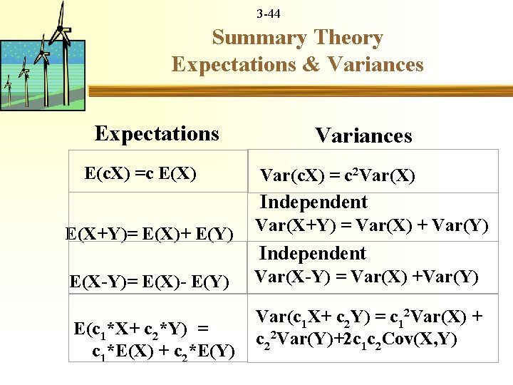
3 -44 Summary Theory Expectations & Variances Expectations Variances E(c. X) =c E(X) E(X+Y)= E(X)+ E(Y) E(X-Y)= E(X)- E(Y) E(c 1*X+ c 2*Y) = c 1*E(X) + c 2*E(Y) Var(c. X) = c 2 Var(X) Independent Var(X+Y) = Var(X) + Var(Y) Independent Var(X-Y) = Var(X) +Var(Y) Var(c 1 X+ c 2 Y) = c 12 Var(X) + c 22 Var(Y)+2 c 1 c 2 Cov(X, Y)

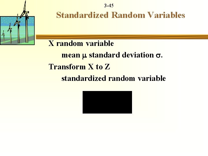
3 -45 Standardized Random Variables X random variable mean standard deviation . Transform X to Z standardized random variable

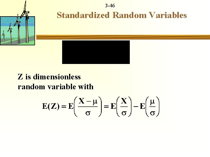
3 -46 Standardized Random Variables Z is dimensionless random variable with

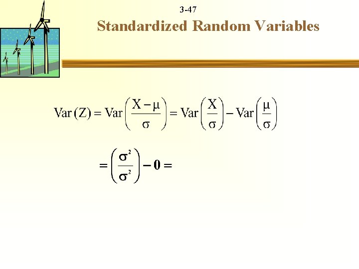
3 -47 Standardized Random Variables

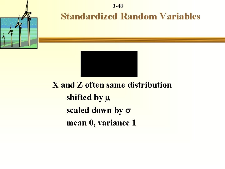
3 -48 Standardized Random Variables X and Z often same distribution shifted by scaled down by mean 0, variance 1

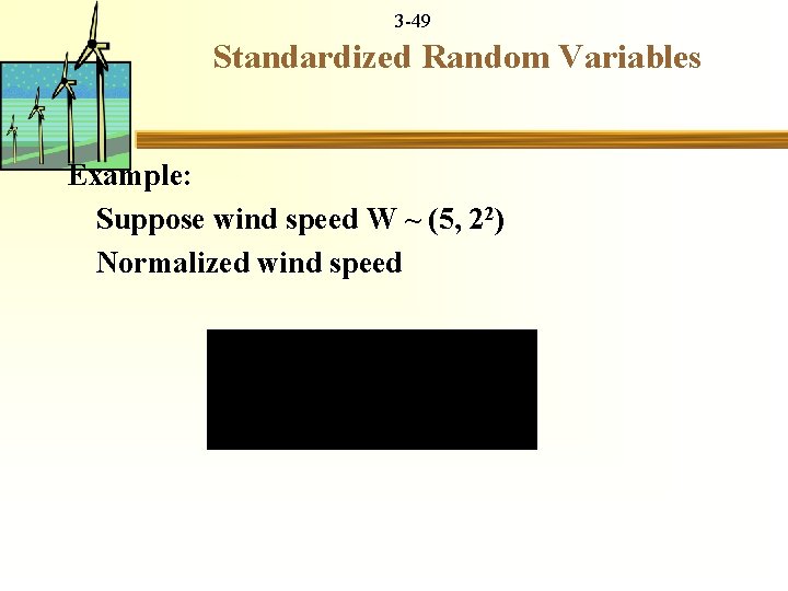
3 -49 Standardized Random Variables Example: Suppose wind speed W ~ (5, 22) Normalized wind speed

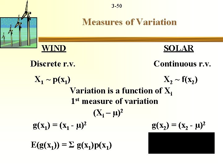
3 -50 Measures of Variation WIND SOLAR Discrete r. v. Continuous r. v. X 1 ~ p(x 1) X 2 ~ f(x 2) Variation is a function of Xi 1 st measure of variation (Xi – µ)2 g(x 1) = (x 1 - µ)2 g(x 2) = (x 2 - µ)2 E(g(x 1)) = Σ g(x 1)p(x 1)

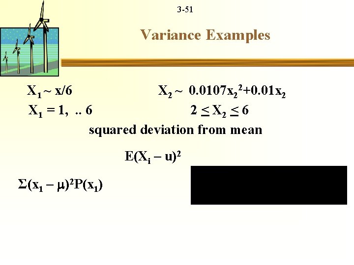
3 -51 Variance Examples X 1 ~ x/6 X 2 ~ 0. 0107 x 22+0. 01 x 2 X 1 = 1, . . 6 2 < X 2 < 6 squared deviation from mean E(Xi – u)2 Σ(x 1 – )2 P(x 1)

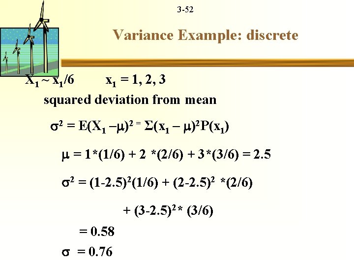
3 -52 Variance Example: discrete X 1 ~ x 1/6 x 1 = 1, 2, 3 squared deviation from mean 2 = E(X 1 – )2 = Σ(x 1 – )2 P(x 1) = 1*(1/6) + 2 *(2/6) + 3*(3/6) = 2. 5 2 = (1 -2. 5)2(1/6) + (2 -2. 5)2 *(2/6) + (3 -2. 5)2* (3/6) = 0. 58 = 0. 76

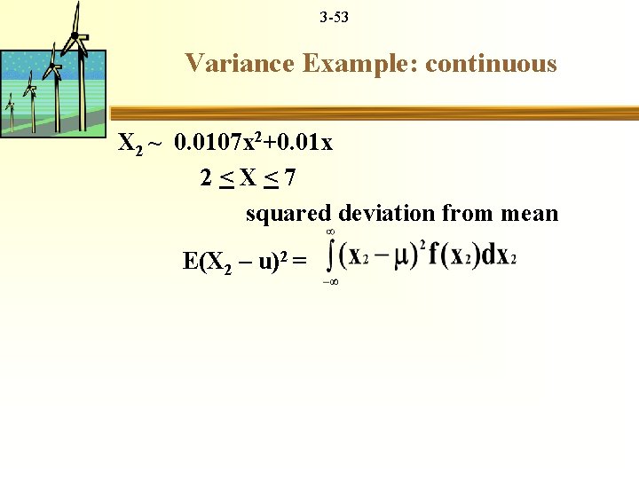
3 -53 Variance Example: continuous X 2 ~ 0. 0107 x 2+0. 01 x 2 < X < 7 squared deviation from mean E(X 2 – u)2 =

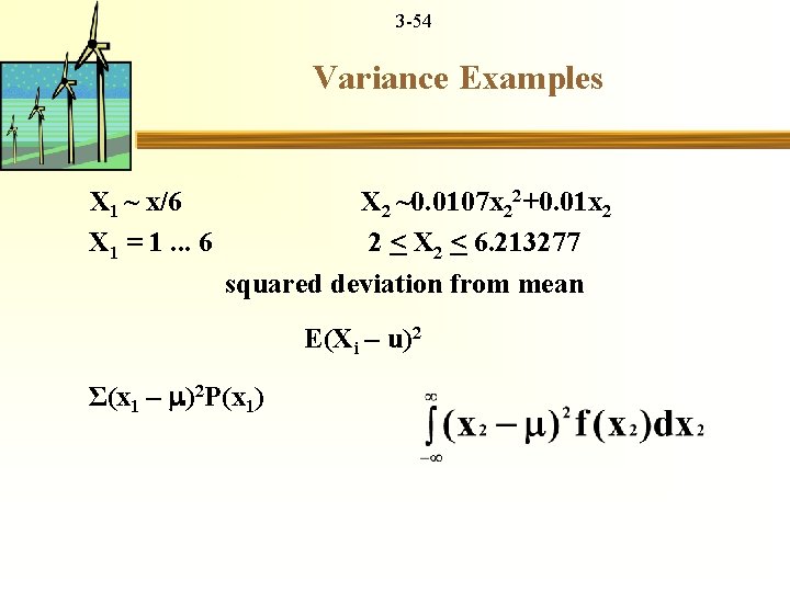
3 -54 Variance Examples X 1 ~ x/6 X 2 ~0. 0107 x 22+0. 01 x 2 X 1 = 1. . . 6 2 < X 2 < 6. 213277 squared deviation from mean E(Xi – u)2 Σ(x 1 – )2 P(x 1)

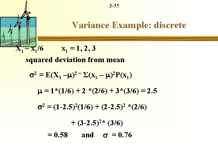
3 -55 Variance Example: discrete X 1 ~ x 1/6 x 1 = 1, 2, 3 squared deviation from mean 2 = E(X 1 – )2 = Σ(x 1 – )2 P(x 1) = 1*(1/6) + 2 *(2/6) + 3*(3/6) = 2. 5 2 = (1 -2. 5)2(1/6) + (2 -2. 5)2 *(2/6) + (3 -2. 5)2* (3/6) = 0. 58 and = 0. 76

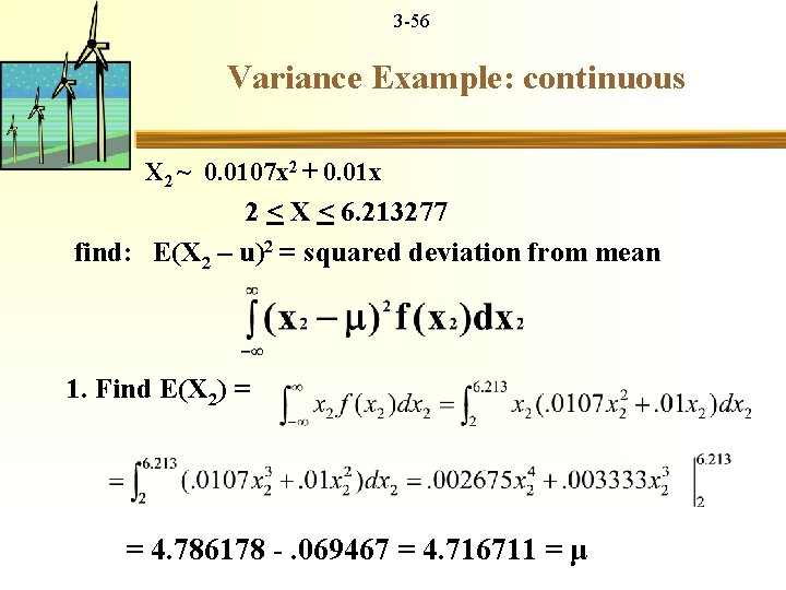
3 -56 Variance Example: continuous X 2 ~ 0. 0107 x 2 + 0. 01 x 2 < X < 6. 213277 find: E(X 2 – u)2 = squared deviation from mean 1. Find E(X 2) = = 4. 786178 -. 069467 = 4. 716711 = μ

3 -57 Variance Example: continuous 2. Find Var(X 2) = E[(X 2 – μ)2] =

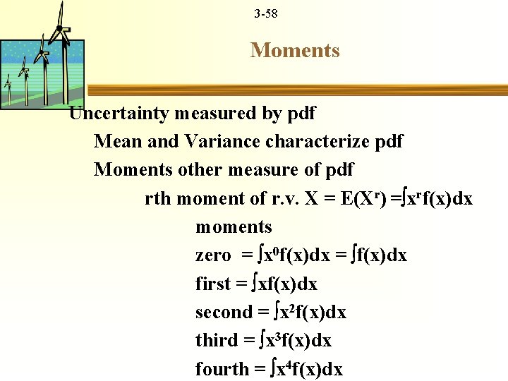
3 -58 Moments Uncertainty measured by pdf Mean and Variance characterize pdf Moments other measure of pdf rth moment of r. v. X = E(Xr) = xrf(x)dx moments zero = x 0 f(x)dx = f(x)dx first = xf(x)dx second = x 2 f(x)dx third = x 3 f(x)dx fourth = x 4 f(x)dx

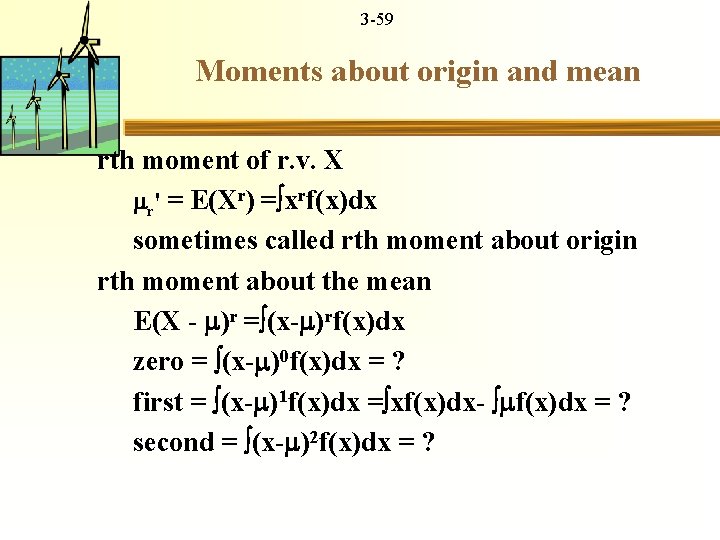
3 -59 Moments about origin and mean rth moment of r. v. X r' = E(Xr) = xrf(x)dx sometimes called rth moment about origin rth moment about the mean E(X - )r = (x- )rf(x)dx zero = (x- )0 f(x)dx = ? first = (x- )1 f(x)dx = xf(x)dx- f(x)dx = ? second = (x- )2 f(x)dx = ?

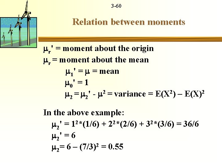
3 -60 Relation between moments r' = moment about the origin r = moment about the mean 1' = = mean 0' = 1 2 = 2' - 2 = variance = E(X 2) – E(X)2 In the above example: 2' = 12*(1/6) + 22*(2/6) + 32*(3/6) = 36/6 2' = 6 2= 6 – (7/3)2 = 0. 55

3 -61 th Show 0, 1, 2, 3, 4 moment and moment about mean for continuous variable X 2 above Verify 2 = 2' - 2 = variance = E(X 2) – E(X)2

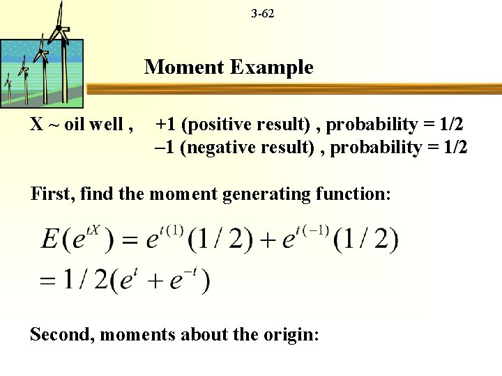
3 -62 Moment Example X ~ oil well , +1 (positive result) , probability = 1/2 – 1 (negative result) , probability = 1/2 First, find the moment generating function: Second, moments about the origin:

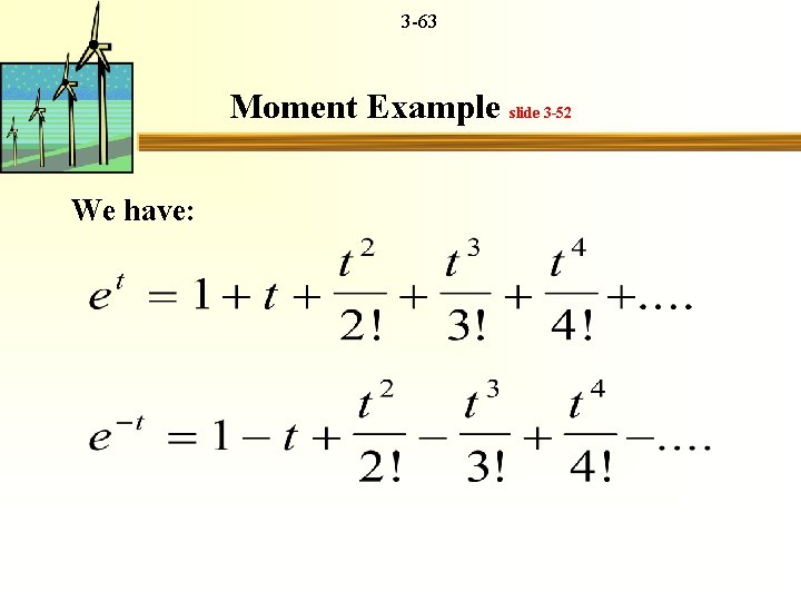
3 -63 Moment Example slide 3 -52 We have:

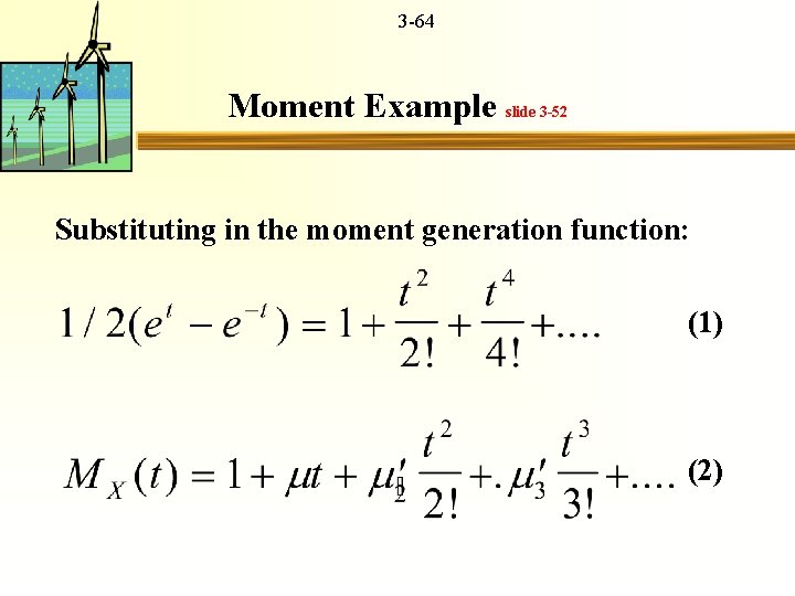
3 -64 Moment Example slide 3 -52 Substituting in the moment generation function: (1) (2)

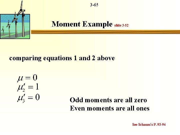
3 -65 Moment Example slide 3 -52 comparing equations 1 and 2 above Odd moments are all zero Even moments are all ones See Schaum’s P. 93 -94

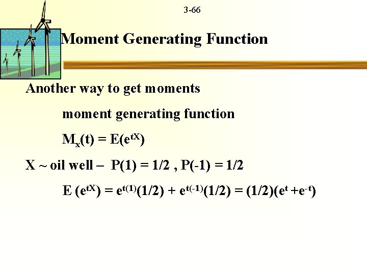
3 -66 Moment Generating Function Another way to get moments moment generating function Mx(t) = E(et. X) X ~ oil well – P(1) = 1/2 , P(-1) = 1/2 E (et. X) = et(1)(1/2) + et(-1)(1/2) = (1/2)(et +e-t)

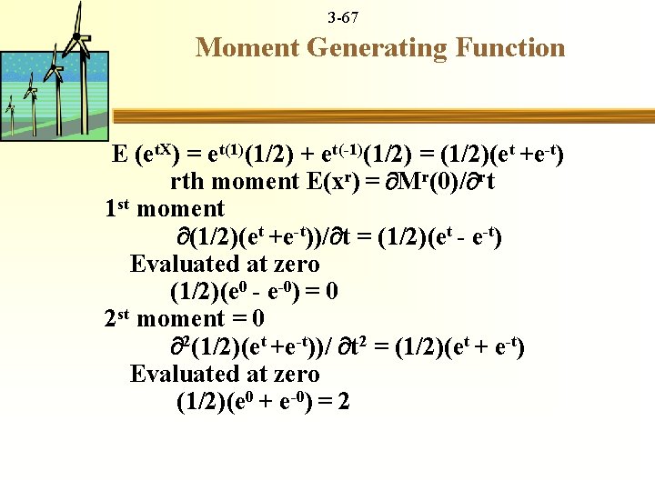
3 -67 Moment Generating Function E (et. X) = et(1)(1/2) + et(-1)(1/2) = (1/2)(et +e-t) rth moment E(xr) = Mr(0)/ rt 1 st moment (1/2)(et +e-t))/ t = (1/2)(et - e-t) Evaluated at zero (1/2)(e 0 - e-0) = 0 2 st moment = 0 2(1/2)(et +e-t))/ t 2 = (1/2)(et + e-t) Evaluated at zero (1/2)(e 0 + e-0) = 2

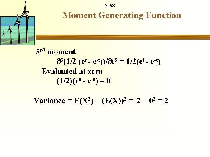
3 -68 Moment Generating Function 3 rd moment 3(1/2 (et - e-t))/ t 3 = 1/2(et - e-t) Evaluated at zero (1/2)(e 0 - e-0) = 0 Variance = E(X 2) – (E(X))2 = 2 – 02 = 2

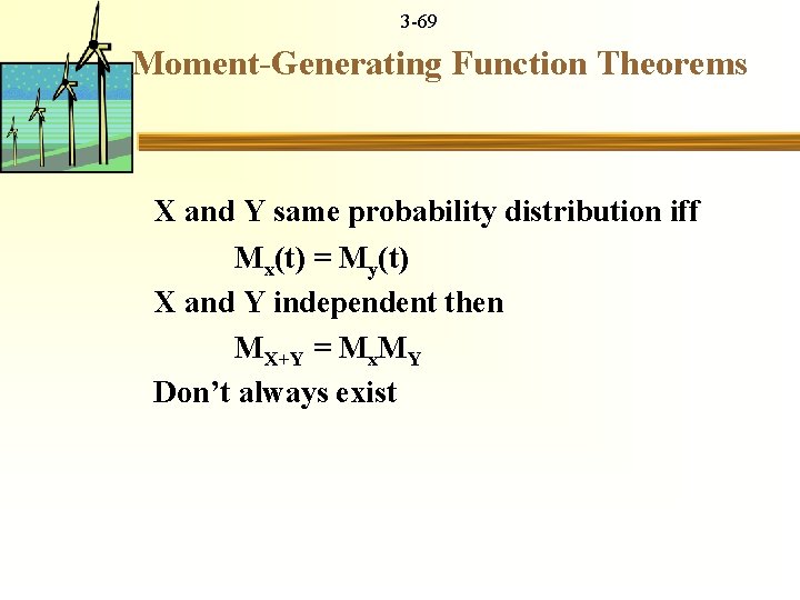
3 -69 Moment-Generating Function Theorems X and Y same probability distribution iff Mx(t) = My(t) X and Y independent then MX+Y = Mx. MY Don’t always exist

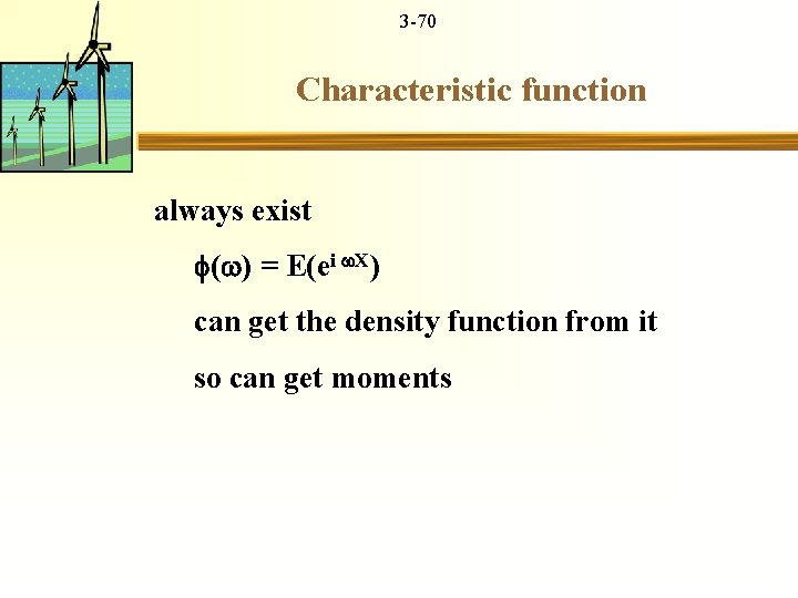
3 -70 Characteristic function always exist ( ) = E(ei X) can get the density function from it so can get moments

3 -71 Joint Distribution Covariance… Covariance is XY = Cov(X, Y) = E[(X- X)(Y- Y)] = E(X, Y) – E(X)E(Y) Using the joint density function f(x, y)

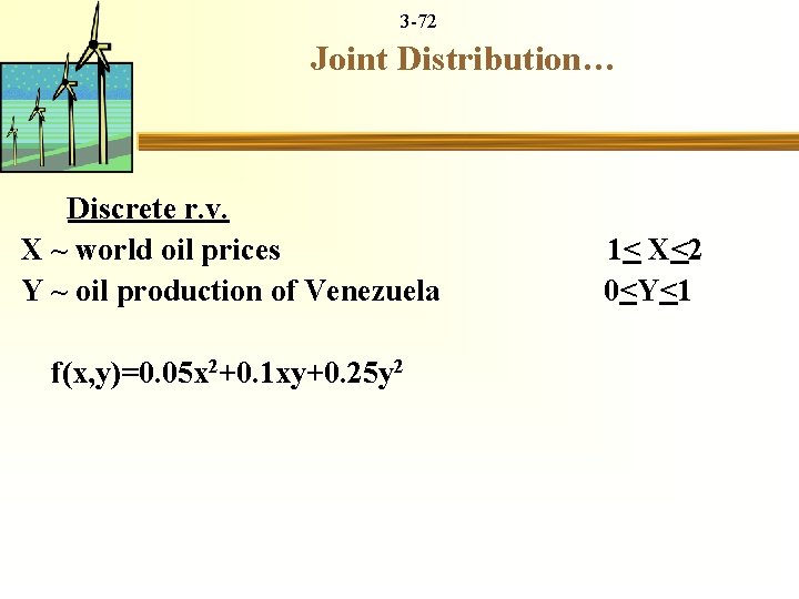
3 -72 Joint Distribution… Discrete r. v. X ~ world oil prices 1< X<2 Y ~ oil production of Venezuela 0<Y<1 f(x, y)=0. 05 x 2+0. 1 xy+0. 25 y 2

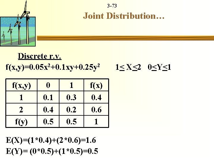
3 -73 Joint Distribution… Discrete r. v. f(x, y)=0. 05 x 2+0. 1 xy+0. 25 y 2 1< X<2 0<Y<1 f(x, y) 0 1 f(x) 1 0. 3 0. 4 2 0. 4 0. 2 0. 6 f(y) 0. 5 1 E(X)=(1*0. 4)+(2*0. 6)=1. 6 E(Y)= (0*0. 5)+(1*0. 5)=0. 5

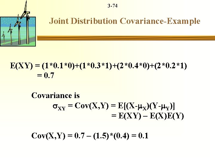
3 -74 Joint Distribution Covariance-Example E(XY) = (1*0. 1*0)+(1*0. 3*1)+(2*0. 4*0)+(2*0. 2*1) = 0. 7 Covariance is XY = Cov(X, Y) = E[(X- X)(Y- Y)] = E(XY) – E(X)E(Y) Cov(X, Y) = 0. 7 – (1. 5)*(0. 4) = 0. 1

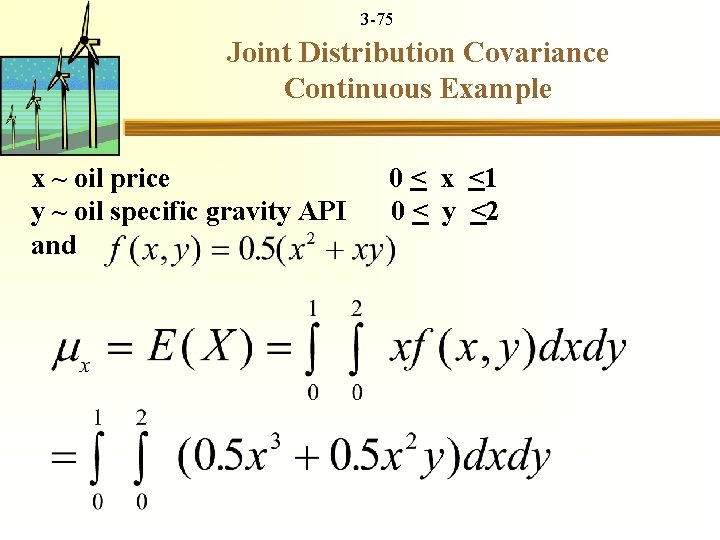
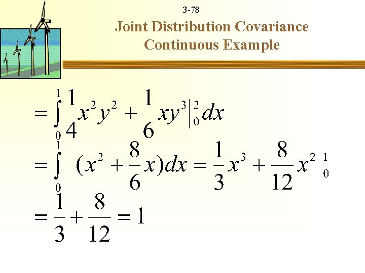
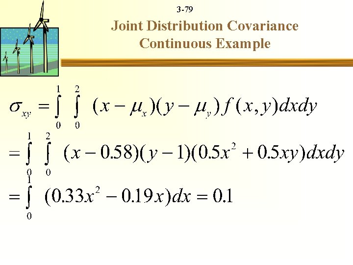
3 -75 Joint Distribution Covariance Continuous Example x ~ oil price 0 < x <1 y ~ oil specific gravity API 0 < y <2 and

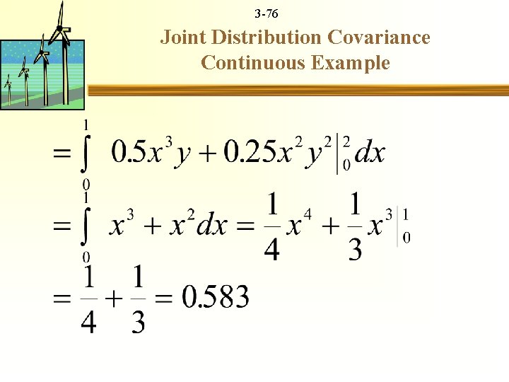
3 -76 Joint Distribution Covariance Continuous Example

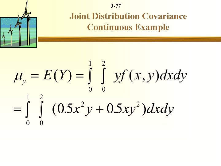
3 -77 Joint Distribution Covariance Continuous Example

3 -78 Joint Distribution Covariance Continuous Example

3 -79 Joint Distribution Covariance Continuous Example

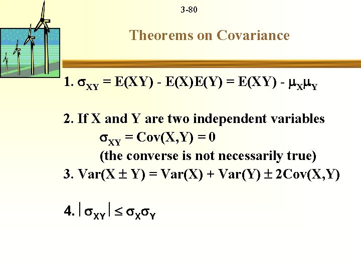
3 -80 Theorems on Covariance 1. XY = E(XY) - E(X)E(Y) = E(XY) - X Y 2. If X and Y are two independent variables XY = Cov(X, Y) = 0 (the converse is not necessarily true) 3. Var(X Y) = Var(X) + Var(Y) 2 Cov(X, Y) 4. XY X Y

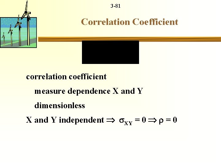
3 -81 Correlation Coefficient correlation coefficient measure dependence X and Y dimensionless X and Y independent XY = 0

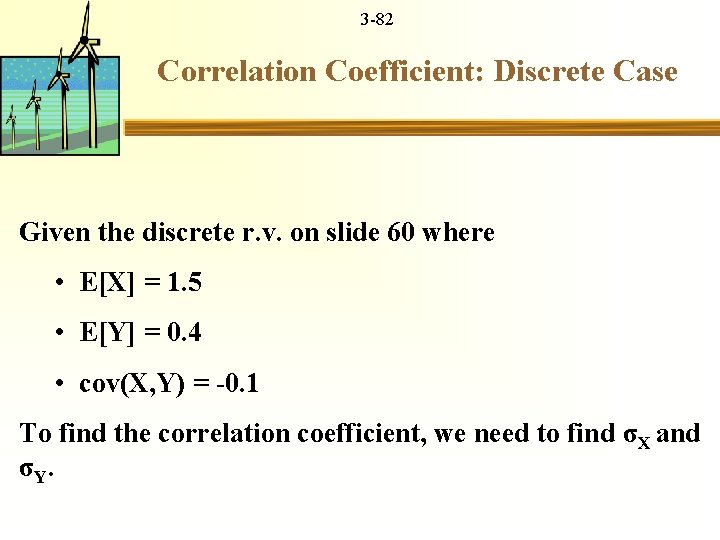
3 -82 Correlation Coefficient: Discrete Case Given the discrete r. v. on slide 60 where • E[X] = 1. 5 • E[Y] = 0. 4 • cov(X, Y) = -0. 1 To find the correlation coefficient, we need to find σX and σ Y.

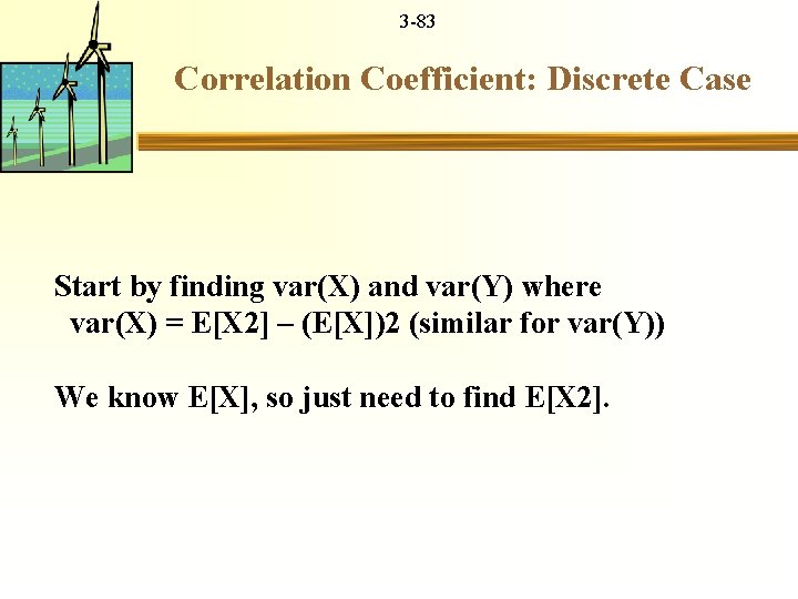
3 -83 Correlation Coefficient: Discrete Case Start by finding var(X) and var(Y) where var(X) = E[X 2] – (E[X])2 (similar for var(Y)) We know E[X], so just need to find E[X 2].

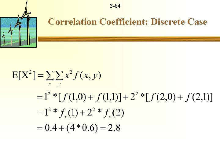
3 -84 Correlation Coefficient: Discrete Case

3 -85 Correlation Coefficient: Discrete Case Using a similar method we find E[Y 2] = 0. 5 We can now figure out var(X) and var(Y) var(X) = 2. 8 – (1. 6)2 = 2. 8 – 2. 56 = 0. 24 and var(Y) = 0. 5 – (0. 5)2 = 0. 25

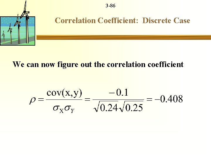
3 -86 Correlation Coefficient: Discrete Case We can now figure out the correlation coefficient

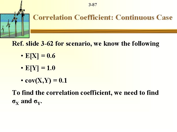
3 -87 Correlation Coefficient: Continuous Case Ref. slide 3 -62 for scenario, we know the following • E[X] = 0. 6 • E[Y] = 1. 0 • cov(X, Y) = 0. 1 To find the correlation coefficient, we need to find σX and σY.

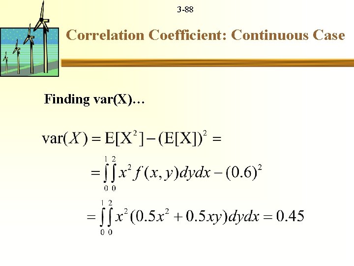
3 -88 Correlation Coefficient: Continuous Case Finding var(X)…

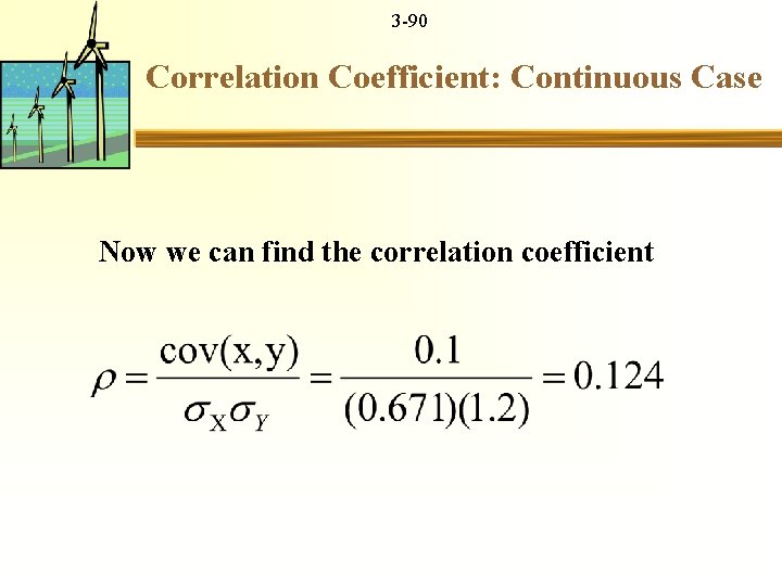
3 -89 Correlation Coefficient: Continuous Case Using a similar technique, we find that var(Y) = 1. 44 Giving us the following • σX = 0. 671 • σY = 1. 2

3 -90 Correlation Coefficient: Continuous Case Now we can find the correlation coefficient

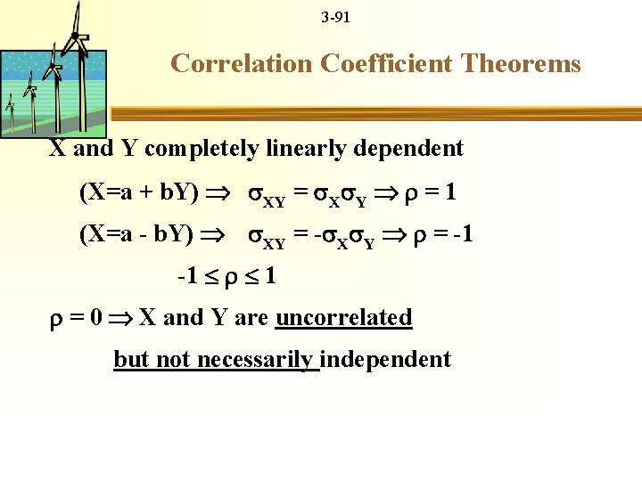
3 -91 Correlation Coefficient Theorems X and Y completely linearly dependent (X=a + b. Y) XY = X Y = 1 (X=a - b. Y) XY = - X Y = -1 -1 1 = 0 X and Y are uncorrelated but not necessarily independent

3 -92 Applications of Correlation important for risk management energy and mineral companies stock investors etc. Negative correlated portfolio of assets reduce business and market risk of companies

3 -93 Conditional Probabilities, Means, and Variances PDQ Oil & Gas acquires new oil &/or natural gas X ~ random variable of oil production Y ~ random variable of gas production Discrete joint probability: P(X, Y) Conditional probability: P(X|Y) Conditional mean: E(X|Y) Conditional variance: 2(X|Y)

3 -94 Discrete Conditional Probabilities P[X|Y] = P(X, Y) = joint probability of X & Y P(Y) marginal probability of Y

3 -95 Discrete Conditional Probabilities P[X=Xi| Y=Yi] = P(X= Xi, Y= Yi) P (Y= Yi) P[X=1000|Y=750] = 0. 25/0. 55 = 0. 455

3 -96 Discrete Conditional Expectation: E[Xi|Y=500] E[Xi|Y=750] E[X|Y=Yi] = ∑ Xi * P[X=Xi | Y=Yi] E[X|Y=500] = 2000(. 10/. 45)+1000(. 10/. 45)+500(. 25/. 45) = 944. 44 bbl E[X|Y=750] = 2000(0. 5/. 55)+1000(. 25/. 55)+500(. 25/. 55) = 863. 64 bbl

3 -97 Discrete Conditional Variance: Var[X|Y=750] Var[X|Y=500] Var [X|Y=Yi] = ∑(X- E[X|Y=Yi])2 * P[X=Xi | Y=Yi] Var [X|Y=500] = (2000 -944. 44)2 (. 10/. 45) + (1000 -944. 44)2 *(. 10/. 45) + (500 -944. 44)2 (. 25/. 45) = 358, 024 bbl Cond. St. Dev. [X | Y=500] = (358, 024)0. 5 = 598. 3 bbl

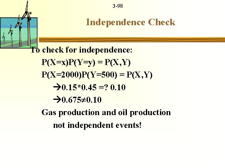
3 -98 Independence Check To check for independence: P(X=x)P(Y=y) = P(X, Y) P(X=2000)P(Y=500) = P(X, Y) 0. 15*0. 45 =? 0. 10 0. 675 0. 10 Gas production and oil production not independent events!

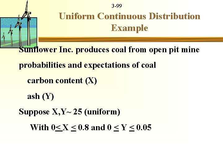
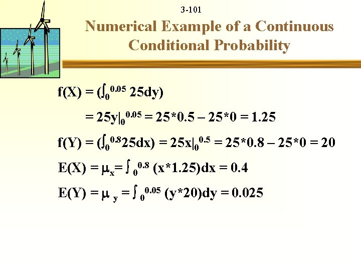
3 -99 Uniform Continuous Distribution Example Sunflower Inc. produces coal from open pit mine probabilities and expectations of coal carbon content (X) ash (Y) Suppose X, Y~ 25 (uniform) With 0< X < 0. 8 and 0 < Y < 0. 05

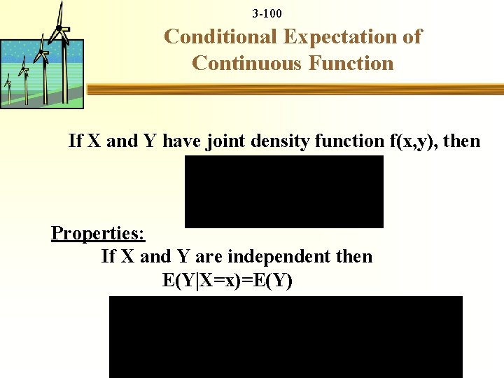
3 -100 Conditional Expectation of Continuous Function If X and Y have joint density function f(x, y), then Properties: If X and Y are independent then E(Y X=x)=E(Y)

3 -101 Numerical Example of a Continuous Conditional Probability f(X) = ( 00. 05 25 dy) = 25 y|00. 05 = 25*0. 5 – 25*0 = 1. 25 f(Y) = ( 00. 825 dx) = 25 x|00. 5 = 25*0. 8 – 25*0 = 20 E(X) = x= 00. 8 (x*1. 25)dx = 0. 4 E(Y) = y = 00. 05 (y*20)dy = 0. 025

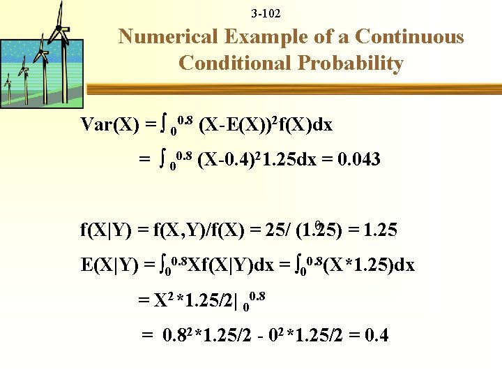
3 -102 Numerical Example of a Continuous Conditional Probability Var(X) = 00. 8 (X-E(X))2 f(X)dx = 00. 8 (X-0. 4)21. 25 dx = 0. 043 0 f(X|Y) = f(X, Y)/f(X) = 25/ (1. 25) = 1. 25 E(X|Y) = 00. 8 Xf(X|Y)dx = 00. 8(X*1. 25)dx = X 2*1. 25/2| 00. 8 2*1. 25/2 - 02*1. 25/2 = 0. 4 = 0. 8

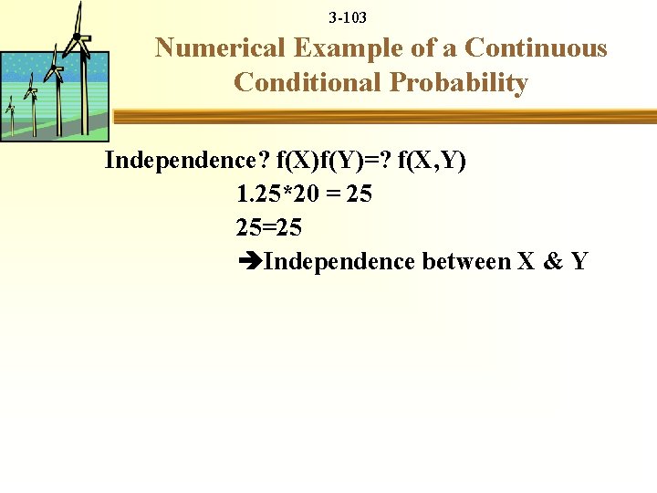
3 -103 Numerical Example of a Continuous Conditional Probability Independence? f(X)f(Y)=? f(X, Y) 1. 25*20 = 25 25=25 Independence between X & Y

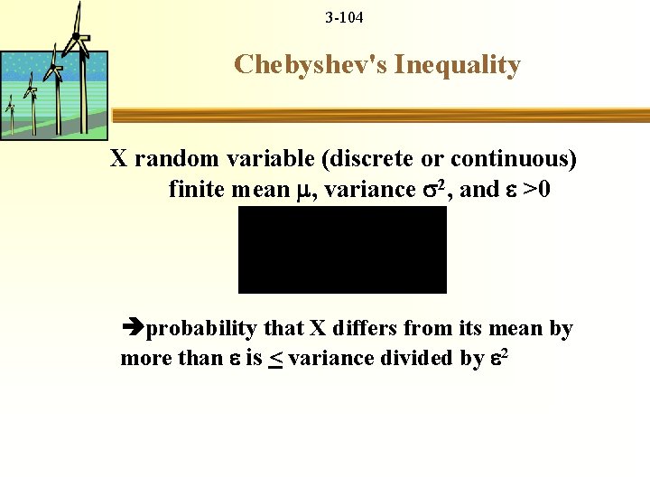
3 -104 Chebyshev's Inequality X random variable (discrete or continuous) finite mean , variance 2, and >0 probability that X differs from its mean by more than is < variance divided by 2

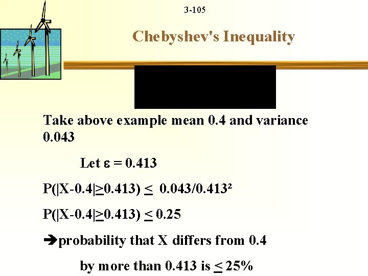
3 -105 Chebyshev's Inequality Take above example mean 0. 4 and variance 0. 043 Let = 0. 413 P(|X-0. 4|>0. 413) < 0. 043/0. 413² P(|X-0. 4|>0. 413) < 0. 25 probability that X differs from 0. 4 by more than 0. 413 is < 25%

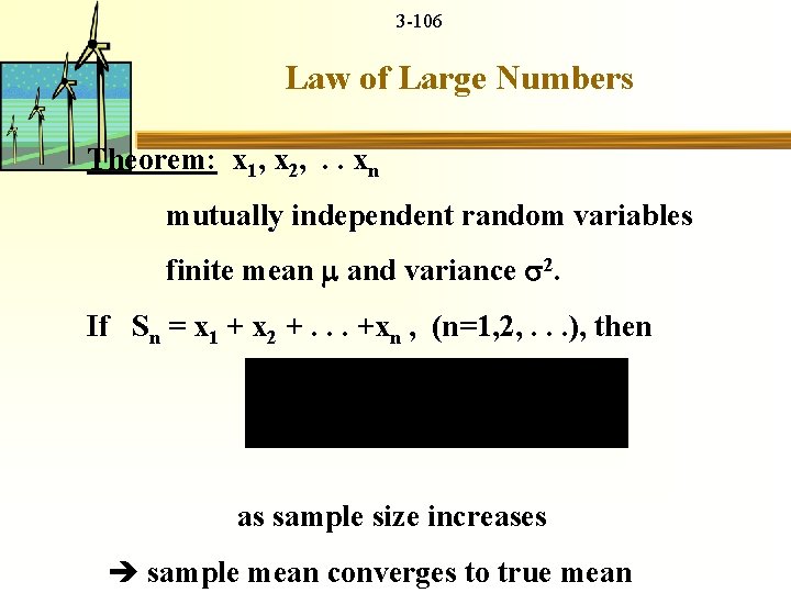
3 -106 Law of Large Numbers Theorem: x 1, x 2, . . xn mutually independent random variables finite mean and variance 2. If Sn = x 1 + x 2 +. . . +xn , (n=1, 2, . . . ), then as sample size increases è sample mean converges to true mean

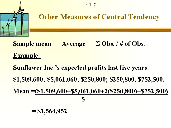
3 -107 Other Measures of Central Tendency Sample mean = Average = S Obs. / # of Obs. Example: Sunflower Inc. ’s expected profits last five years: $1, 509, 600; $5, 061, 060; $250, 800, $752, 500. Mean =($1, 509, 600+$5, 061, 060+2($250, 800)+$752, 500) 5 = $1, 564, 952

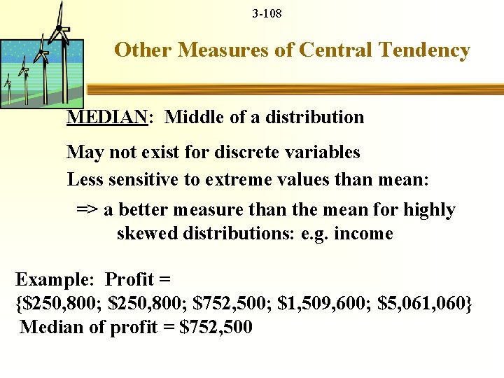
3 -108 Other Measures of Central Tendency MEDIAN: Middle of a distribution May not exist for discrete variables Less sensitive to extreme values than mean: => a better measure than the mean for highly skewed distributions: e. g. income Example: Profit = {$250, 800; $752, 500; $1, 509, 600; $5, 061, 060} Median of profit = $752, 500

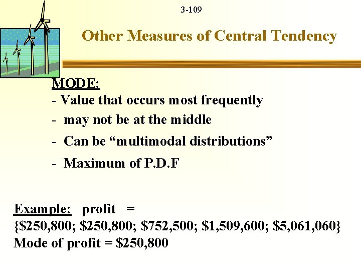
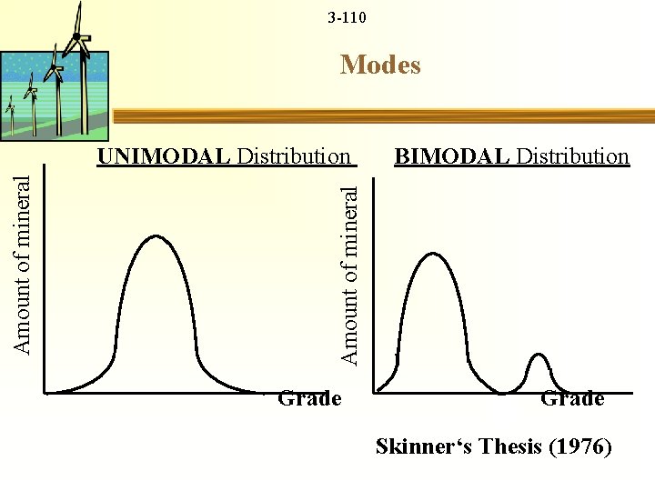
3 -109 Other Measures of Central Tendency MODE: - Value that occurs most frequently - may not be at the middle - Can be “multimodal distributions” - Maximum of P. D. F Example: profit = {$250, 800; $752, 500; $1, 509, 600; $5, 061, 060} Mode of profit = $250, 800

3 -110 Modes Amount of mineral UNIMODAL Distribution BIMODAL Distribution Grade Skinner‘s Thesis (1976)

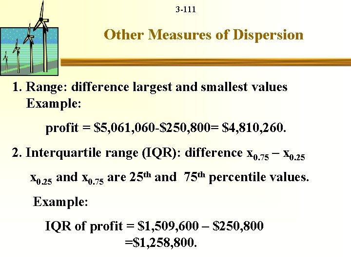
3 -111 Other Measures of Dispersion 1. Range: difference largest and smallest values Example: profit = $5, 061, 060 -$250, 800= $4, 810, 260. 2. Interquartile range (IQR): difference x 0. 75 – x 0. 25 and x 0. 75 are 25 th and 75 th percentile values. Example: IQR of profit = $1, 509, 600 – $250, 800 =$1, 258, 800.

3 -112 Other Measures of Dispersion 3. Mean Deviation (MD): E( X- ). Example: Add a mineral economic example of mean deviation for a continuous and discrete r. v.

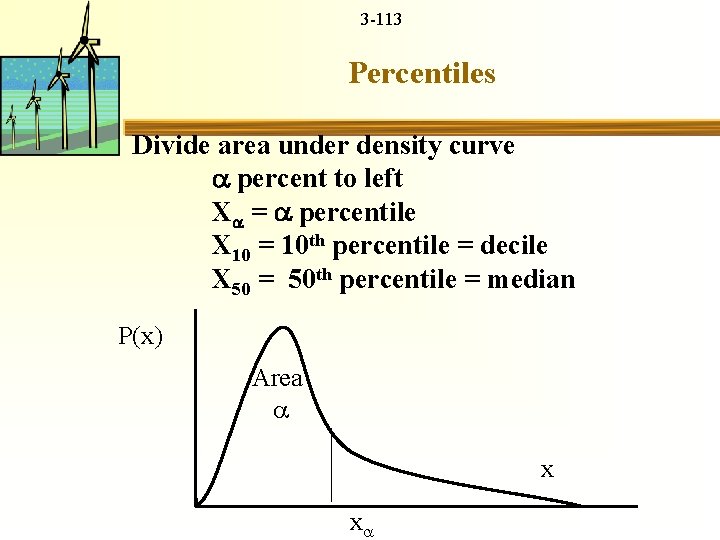
3 -113 Percentiles Divide area under density curve percent to left X = percentile X 10 = 10 th percentile = decile X 50 = 50 th percentile = median P(x) Area x x

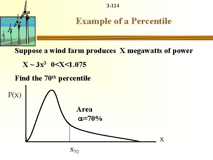
3 -114 Example of a Percentile Suppose a wind farm produces X megawatts of power X ~ 3 x 3 0<X<1. 075 Find the 70 th percentile P(x) Area =70% x x 70

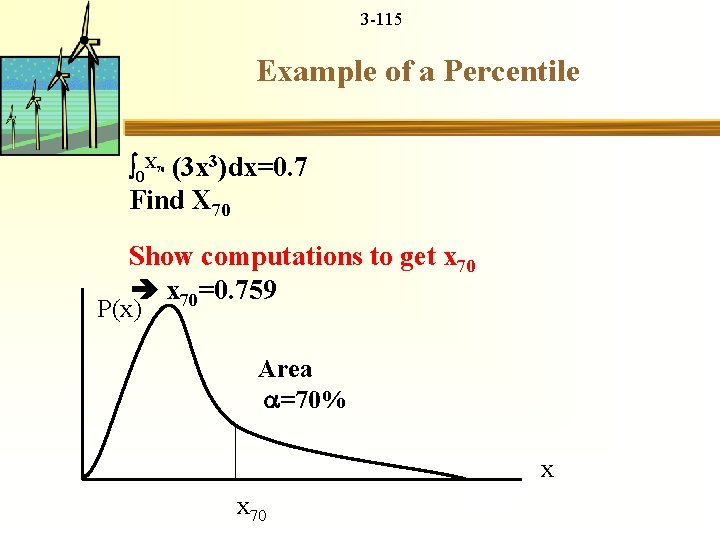
3 -115 Example of a Percentile 0 X (3 x 3)dx=0. 7 70 Find X 70 Show computations to get x 70=0. 759 P(x) Area =70% x x 70

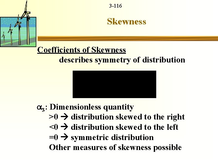
3 -116 Skewness Coefficients of Skewness describes symmetry of distribution 3: Dimensionless quantity >0 distribution skewed to the right <0 distribution skewed to the left =0 symmetric distribution Other measures of skewness possible

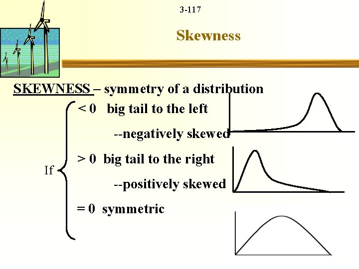
3 -117 Skewness SKEWNESS – symmetry of a distribution < 0 big tail to the left --negatively skewed If > 0 big tail to the right --positively skewed = 0 symmetric

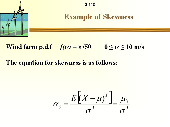
3 -118 Example of Skewness Wind farm p. d. f f(w) = w/50 0 ≤ w ≤ 10 m/s The equation for skewness is as follows:

3 -119 Example of Skewness Recall from slide 13, E[w] = 6. 67 m/s We need to find E[(W – E[W])2].

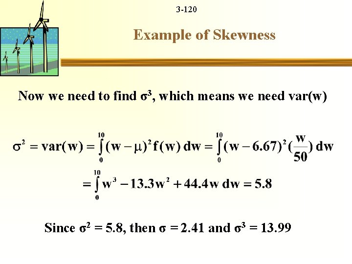
3 -120 Example of Skewness Now we need to find σ3, which means we need var(w) Since σ2 = 5. 8, then σ = 2. 41 and σ3 = 13. 99

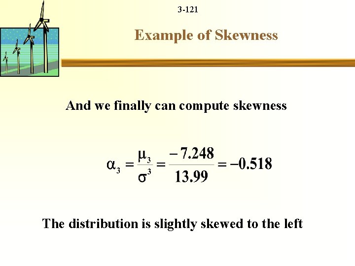
3 -121 Example of Skewness And we finally can compute skewness The distribution is slightly skewed to the left

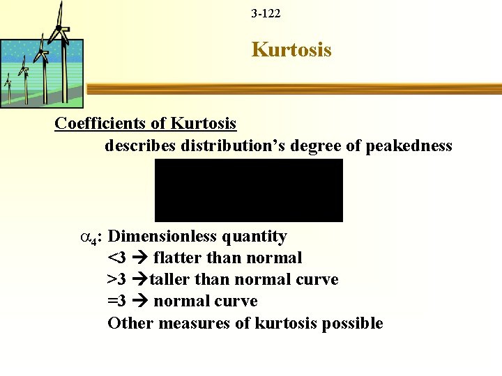
3 -122 Kurtosis Coefficients of Kurtosis describes distribution’s degree of peakedness 4: Dimensionless quantity <3 flatter than normal >3 taller than normal curve =3 normal curve Other measures of kurtosis possible

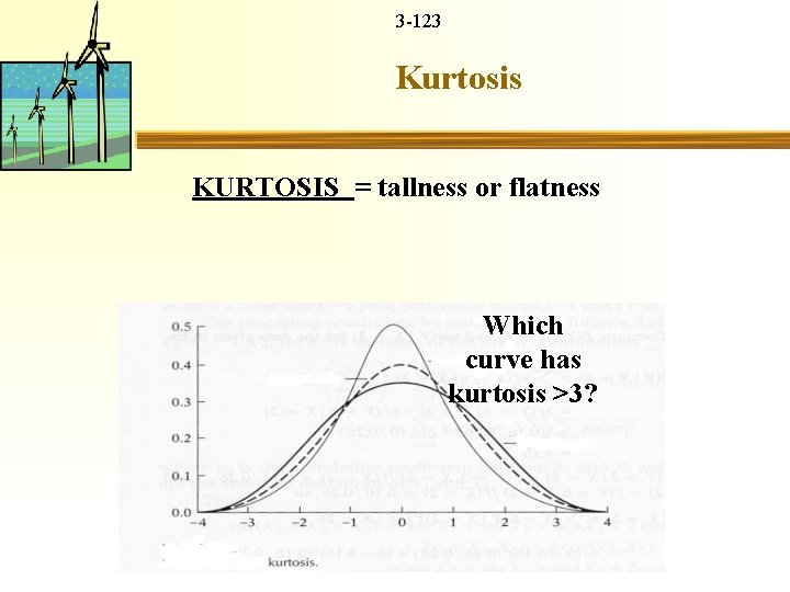
3 -123 Kurtosis KURTOSIS = tallness or flatness Which curve has kurtosis >3?

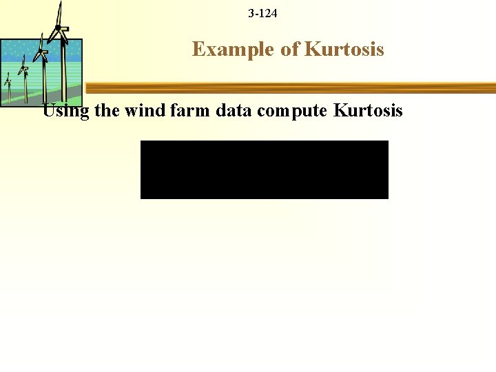
3 -124 Example of Kurtosis Using the wind farm data compute Kurtosis

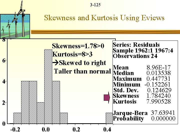
3 -125 Skewness and Kurtosis Using Eviews 8 Skewness=1. 78>0 Series: Residuals Sample 1962: 1 1967: 4 Kurtosis=8>3 Observations 24 Skewed to right Mean 8. 96 E-17 Taller than normal Median 0. 013538 6 Maximum Minimum Std. Dev. Skewness Kurtosis 4 2 0 0. 447731 -0. 152261 0. 124629 1. 784240 7. 990528 Jarque-Bera 37. 63941 Probability 0. 000000 -0. 2 0. 0 0. 2 0. 4

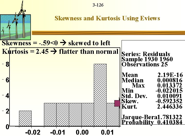
3 -126 Skewness and Kurtosis Using Eviews Skewness = -. 59<0 skewed to left Kurtosis = 2. 45 flatter than normal Series: Residuals Sample 1930 1960 Observations 25 8 Mean Median Max Min Std. Dev. Skew. Kurt. 6 4 2 0 2. 19 E-16 0. 000816 0. 013372 -0. 022015 0. 010091 -0. 592352 2. 446336 Jarque-Bera 1. 781322 Probability 0. 410384 -0. 02 -0. 01 0. 00 0. 01

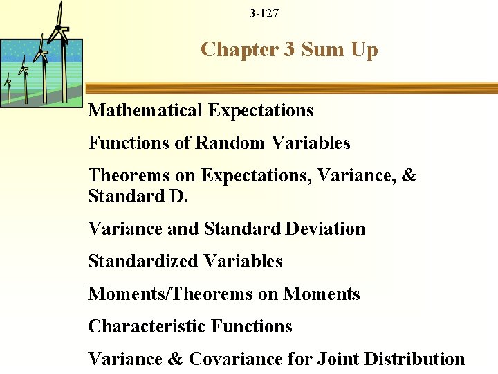
3 -127 Chapter 3 Sum Up Mathematical Expectations Functions of Random Variables Theorems on Expectations, Variance, & Standard D. Variance and Standard Deviation Standardized Variables Moments/Theorems on Moments Characteristic Functions Variance & Covariance for Joint Distribution

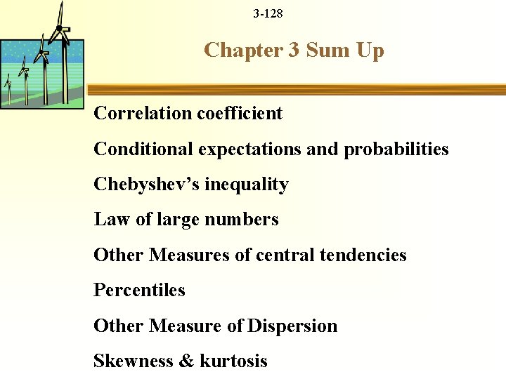
3 -128 Chapter 3 Sum Up Correlation coefficient Conditional expectations and probabilities Chebyshev’s inequality Law of large numbers Other Measures of central tendencies Percentiles Other Measure of Dispersion Skewness & kurtosis