CHAPTER 13 FORECASTING VOLATILITY I In ARMA models
- Slides: 15

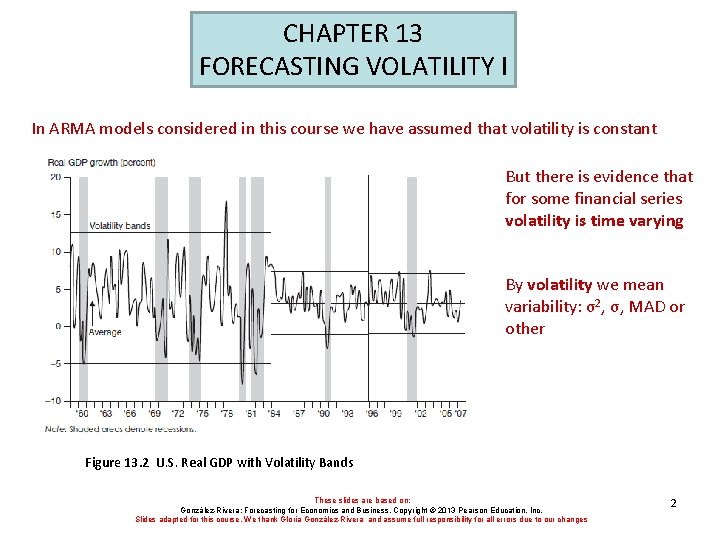
CHAPTER 13 FORECASTING VOLATILITY I In ARMA models considered in this course we have assumed that volatility is constant But there is evidence that for some financial series volatility is time varying By volatility we mean variability: σ2, σ, MAD or other Figure 13. 2 U. S. Real GDP with Volatility Bands These slides are based on: González-Rivera: Forecasting for Economics and Business, Copyright © 2013 Pearson Education, Inc. Slides adapted for this course. We thank Gloria González-Rivera and assume full responsibility for all errors due to our changes 2

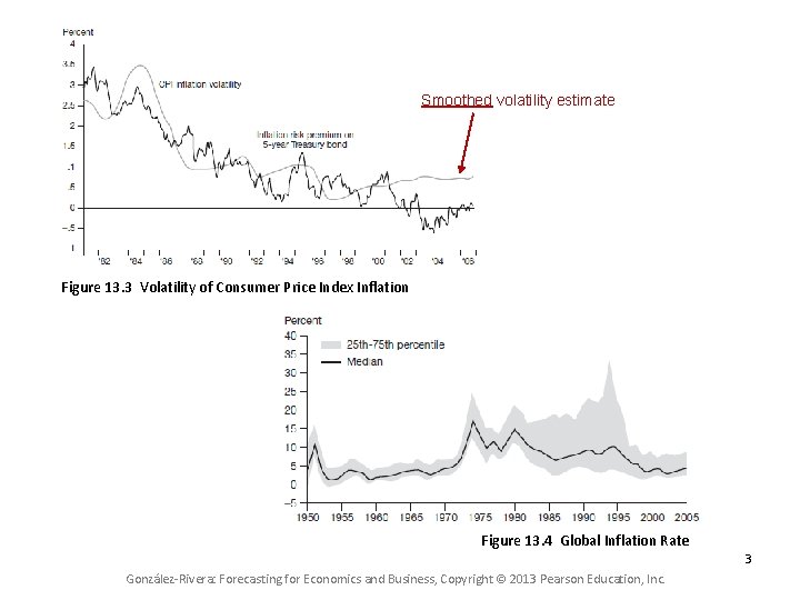
Smoothed volatility estimate Figure 13. 3 Volatility of Consumer Price Index Inflation Figure 13. 4 Global Inflation Rate 3 González-Rivera: Forecasting for Economics and Business, Copyright © 2013 Pearson Education, Inc.

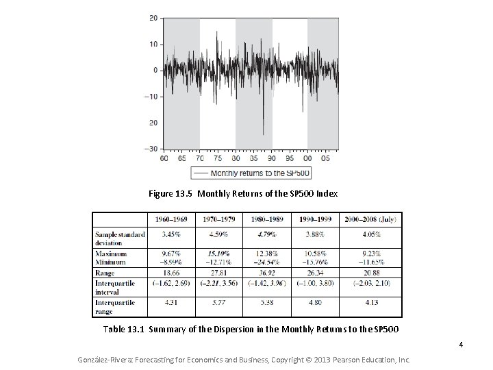
Figure 13. 5 Monthly Returns of the SP 500 Index Table 13. 1 Summary of the Dispersion in the Monthly Returns to the SP 500 4 González-Rivera: Forecasting for Economics and Business, Copyright © 2013 Pearson Education, Inc.

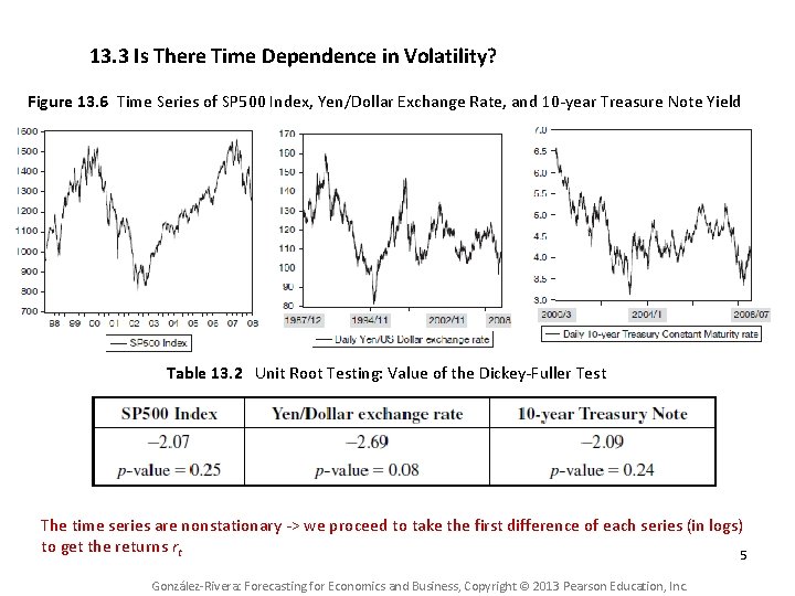
13. 3 Is There Time Dependence in Volatility? Figure 13. 6 Time Series of SP 500 Index, Yen/Dollar Exchange Rate, and 10 -year Treasure Note Yield Table 13. 2 Unit Root Testing: Value of the Dickey-Fuller Test The time series are nonstationary -> we proceed to take the first difference of each series (in logs) to get the returns rt 5 González-Rivera: Forecasting for Economics and Business, Copyright © 2013 Pearson Education, Inc.

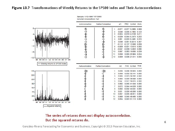
Figure 13. 7 Transformations of Weekly Returns to the SP 500 Index and Their Autocorrelations The series of returns does not display autocorrelation. But the squared returns do. González-Rivera: Forecasting for Economics and Business, Copyright © 2013 Pearson Education, Inc. 6

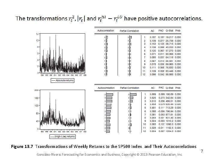
Figure 13. 7 Transformations of Weekly Returns to the SP 500 Index and Their Autocorrelations González-Rivera: Forecasting for Economics and Business, Copyright © 2013 Pearson Education, Inc. 7

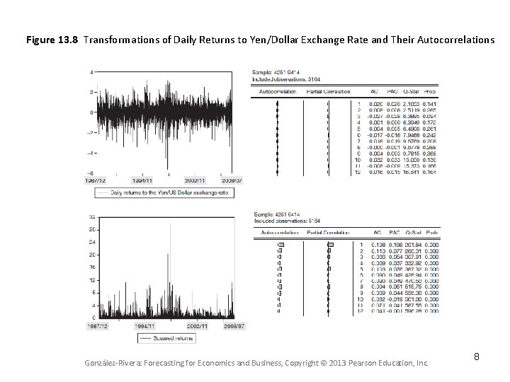
Figure 13. 8 Transformations of Daily Returns to Yen/Dollar Exchange Rate and Their Autocorrelations González-Rivera: Forecasting for Economics and Business, Copyright © 2013 Pearson Education, Inc. 8

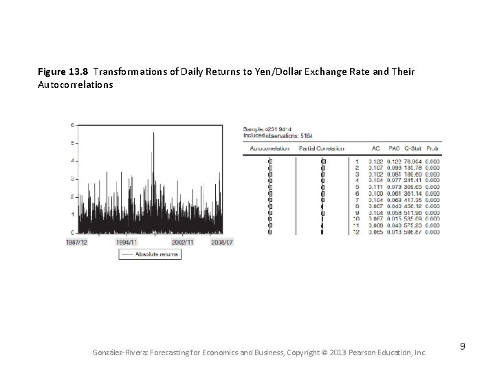
Figure 13. 8 Transformations of Daily Returns to Yen/Dollar Exchange Rate and Their Autocorrelations González-Rivera: Forecasting for Economics and Business, Copyright © 2013 Pearson Education, Inc. 9

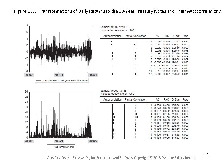
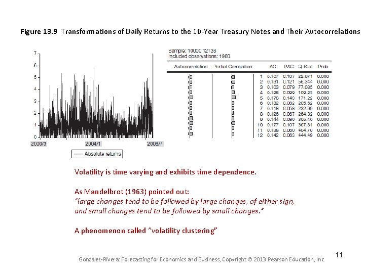
Figure 13. 9 Transformations of Daily Returns to the 10 -Year Treasury Notes and Their Autocorrelations González-Rivera: Forecasting for Economics and Business, Copyright © 2013 Pearson Education, Inc. 10

Figure 13. 9 Transformations of Daily Returns to the 10 -Year Treasury Notes and Their Autocorrelations Volatility is time varying and exhibits time dependence. As Mandelbrot (1963) pointed out: “large changes tend to be followed by large changes, of either sign, and small changes tend to be followed by small changes. ” A phenomenon called “volatility clustering” González-Rivera: Forecasting for Economics and Business, Copyright © 2013 Pearson Education, Inc. 11

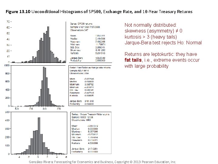
Figure 13. 10 Unconditional Histograms of SP 500, Exchange Rate, and 10 -Year Treasury Returns Not normally distributed: skewness (asymmetry) ≠ 0 kurtosis > 3 (heavy tails) Jarque-Bera test rejects Ho: Normal Returns are leptokurtic: they have fat tails, i. e. , extreme events occur with large probability González-Rivera: Forecasting for Economics and Business, Copyright © 2013 Pearson Education, Inc.

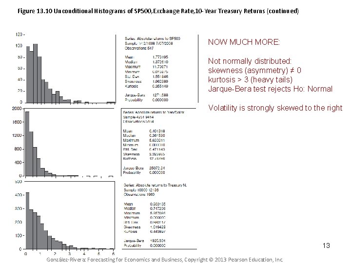
Figure 13. 10 Unconditional Histograms of SP 500, Exchange Rate, 10 -Year Treasury Returns (continued) NOW MUCH MORE: Not normally distributed: skewness (asymmetry) ≠ 0 kurtosis > 3 (heavy tails) Jarque-Bera test rejects Ho: Normal Volatility is strongly skewed to the right 13 González-Rivera: Forecasting for Economics and Business, Copyright © 2013 Pearson Education, Inc.

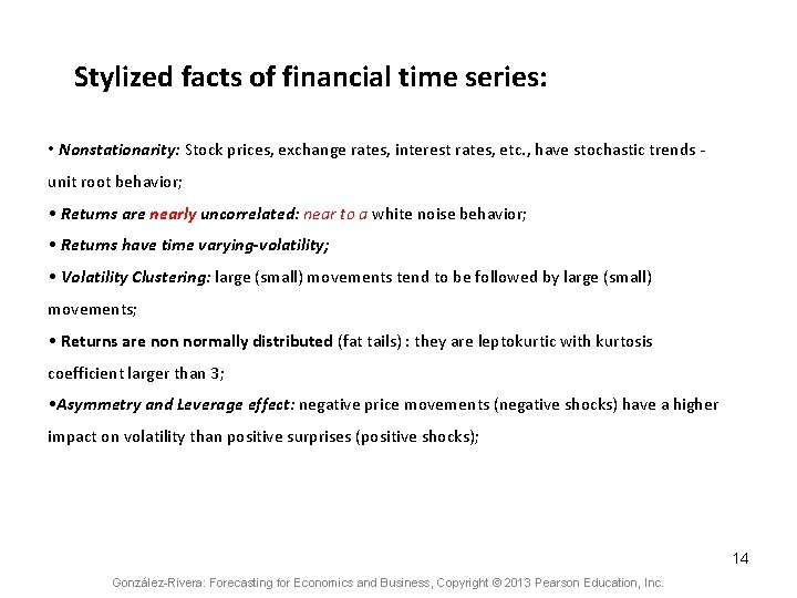
Stylized facts of financial time series: • Nonstationarity: Stock prices, exchange rates, interest rates, etc. , have stochastic trends unit root behavior; • Returns are nearly uncorrelated: near to a white noise behavior; • Returns have time varying-volatility; • Volatility Clustering: large (small) movements tend to be followed by large (small) movements; • Returns are non normally distributed (fat tails) : they are leptokurtic with kurtosis coefficient larger than 3; • Asymmetry and Leverage effect: negative price movements (negative shocks) have a higher impact on volatility than positive surprises (positive shocks); 14 González-Rivera: Forecasting for Economics and Business, Copyright © 2013 Pearson Education, Inc.

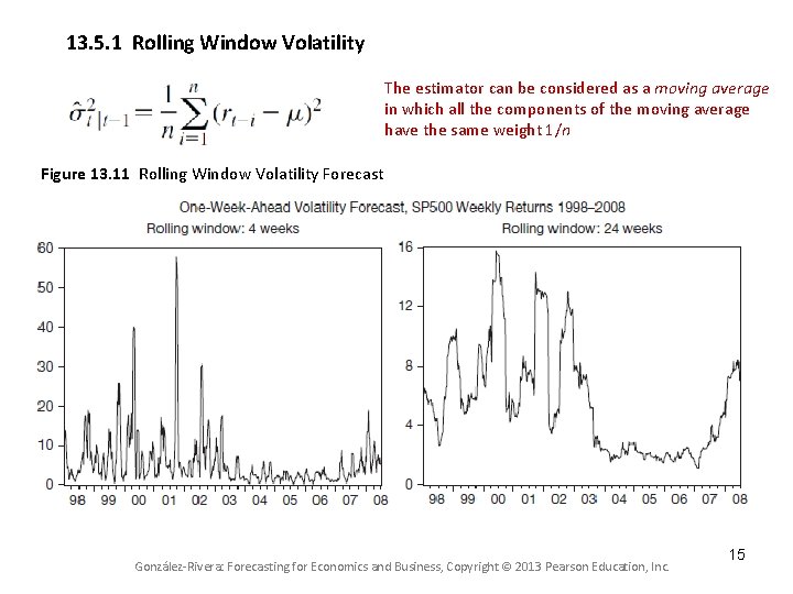
13. 5. 1 Rolling Window Volatility The estimator can be considered as a moving average in which all the components of the moving average have the same weight 1/n Figure 13. 11 Rolling Window Volatility Forecast González-Rivera: Forecasting for Economics and Business, Copyright © 2013 Pearson Education, Inc. 15

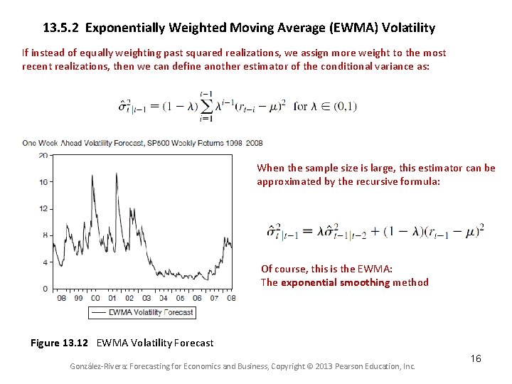
13. 5. 2 Exponentially Weighted Moving Average (EWMA) Volatility If instead of equally weighting past squared realizations, we assign more weight to the most recent realizations, then we can define another estimator of the conditional variance as: When the sample size is large, this estimator can be approximated by the recursive formula: Of course, this is the EWMA: The exponential smoothing method Figure 13. 12 EWMA Volatility Forecast González-Rivera: Forecasting for Economics and Business, Copyright © 2013 Pearson Education, Inc. 16