CHAPTER 13 Design and Analysis of SingleFactor Experiments

CHAPTER 13 Design and Analysis of Single-Factor Experiments: The Analysis of Variance

Learning Objectives • Design and conduct engineering experiments • Understand how the analysis of variance is used to analyze the data • Use multiple comparison procedures • Make decisions about sample size • Understand the difference between fixed and random factors • Estimate variance components • Understand the blocking principle • Design and conduct experiments involving the randomized complete block design

Engineering Experiments • Experiments are a natural part of the engineering decision-making process • Designed to improve the performance of a subset of processes • Processes can be described in terms of controllable variables • Determine which subset has the greatest influence • Such analysis can lead to – Improved process yield – Reduced variability in the process and closer conformance to nominal or target requirements – Reduced cost of operation

Steps In Experimental Design • Usually designed sequentially • Determine which variables are most important • Used to refine the information to determine the critical variables for improving the process • Determine which variables result in the best process performance

Single Factor Experiment • Assume a parameter of interest • Consist of making up several specimens in two samples • Analyzed them using the statistical hypotheses methods • Can say an experiment with single factor – Has two levels of investigations – Levels are called treatments – Treatment has n observations or replicates

Designing Engineering Experiments • More than two levels of the factor • This chapter shows – ANalysis Of VAriance (ANOVA) – Discuss randomization of the experimental runs • Design and analyze experiments with several factors

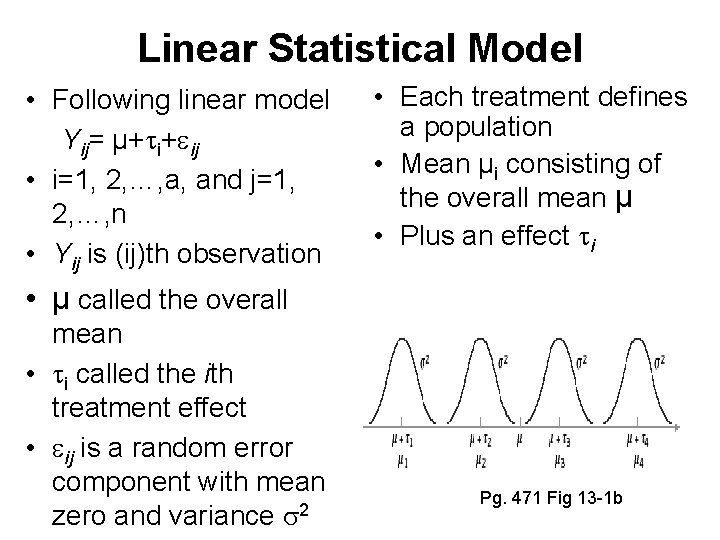
Linear Statistical Model • Following linear model Yij= µ+ i+ ij • i=1, 2, …, a, and j=1, 2, …, n • Yij is (ij)th observation • Each treatment defines a population • Mean µi consisting of the overall mean µ • Plus an effect i • µ called the overall mean • i called the ith treatment effect • ij is a random error component with mean zero and variance 2 Pg. 471 Fig 13 -1 b

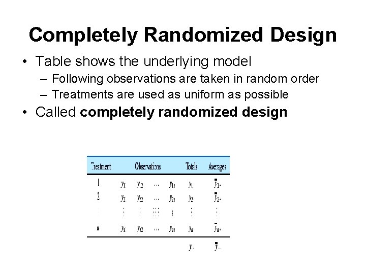
Completely Randomized Design • Table shows the underlying model – Following observations are taken in random order – Treatments are used as uniform as possible • Called completely randomized design

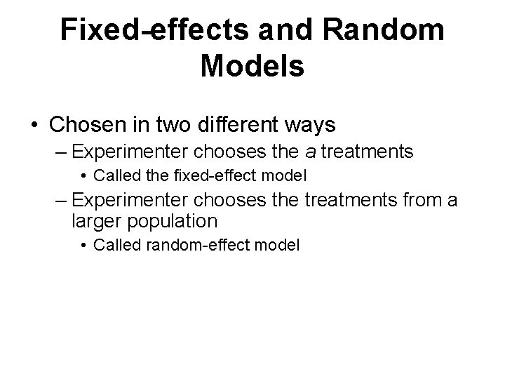
Fixed-effects and Random Models • Chosen in two different ways – Experimenter chooses the a treatments • Called the fixed-effect model – Experimenter chooses the treatments from a larger population • Called random-effect model

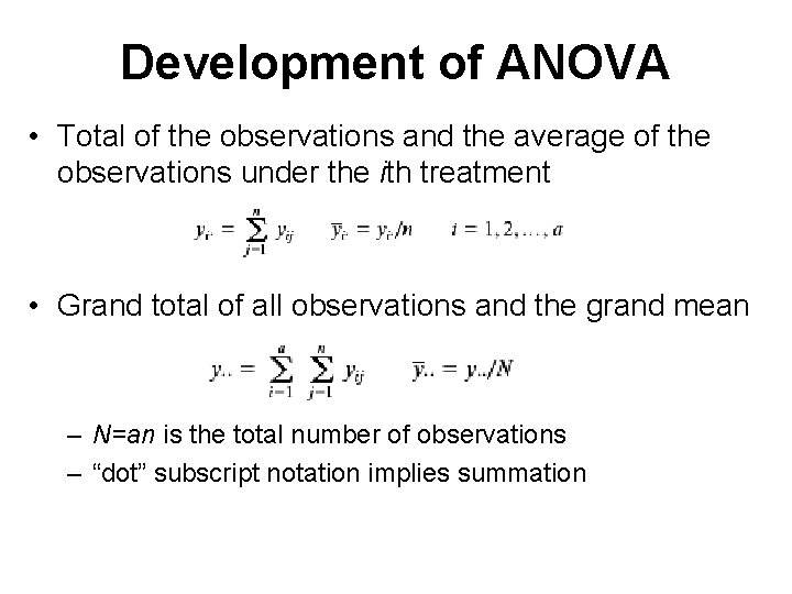
Development of ANOVA • Total of the observations and the average of the observations under the ith treatment • Grand total of all observations and the grand mean – N=an is the total number of observations – “dot” subscript notation implies summation

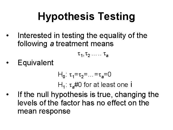
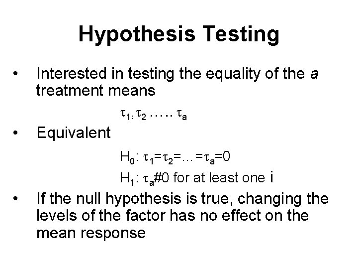
Hypothesis Testing • Interested in testing the equality of the following a treatment means 1, 2 …. . a • Equivalent H 0: 1= 2=…= a=0 H 1: a#0 for at least one i • If the null hypothesis is true, changing the levels of the factor has no effect on the mean response

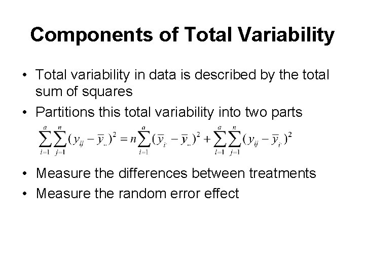
Components of Total Variability • Total variability in data is described by the total sum of squares • Partitions this total variability into two parts • Measure the differences between treatments • Measure the random error effect

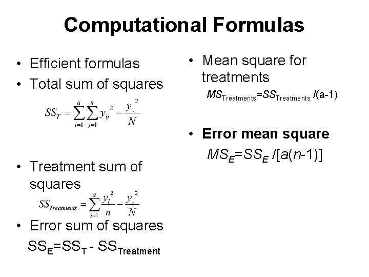
Computational Formulas • Efficient formulas • Total sum of squares • Treatment sum of squares • Error sum of squares SSE=SST - SSTreatment • Mean square for treatments MSTreatments=SSTreatments /(a-1) • Error mean square MSE=SSE /[a(n-1)]

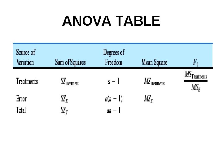
ANOVA TABLE

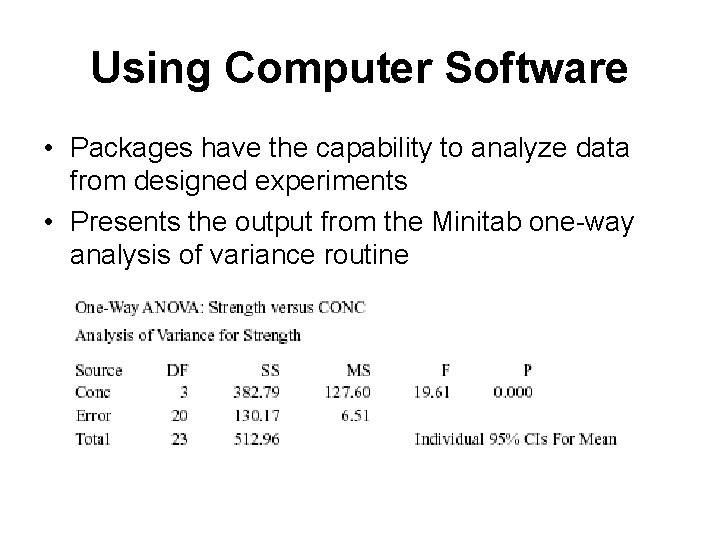
Using Computer Software • Packages have the capability to analyze data from designed experiments • Presents the output from the Minitab one-way analysis of variance routine

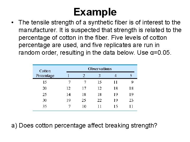
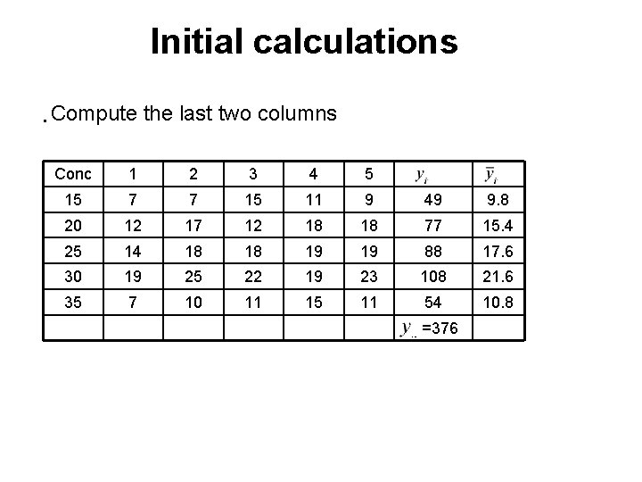
Example • The tensile strength of a synthetic fiber is of interest to the manufacturer. It is suspected that strength is related to the percentage of cotton in the fiber. Five levels of cotton percentage are used, and five replicates are run in random order, resulting in the data below. Use α=0. 05. a) Does cotton percentage affect breaking strength?

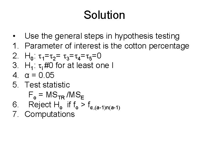
Solution • 1. 2. 3. 4. 5. Use the general steps in hypothesis testing Parameter of interest is the cotton percentage H 0: 1= 2= 3= 4= 5=0 H 1: i #0 for at least one I α = 0. 05 Test statistic Fo = MSTR /MSE 6. Reject Ho if fo > fα, (a-1)n(a-1) 7. Computations

Initial calculations • Compute the last two columns Conc 1 2 3 4 5 15 7 7 15 11 9 49 9. 8 20 12 17 12 18 18 77 15. 4 25 14 18 18 19 19 88 17. 6 30 19 25 22 19 23 108 21. 6 35 7 10 11 15 11 54 10. 8 =376

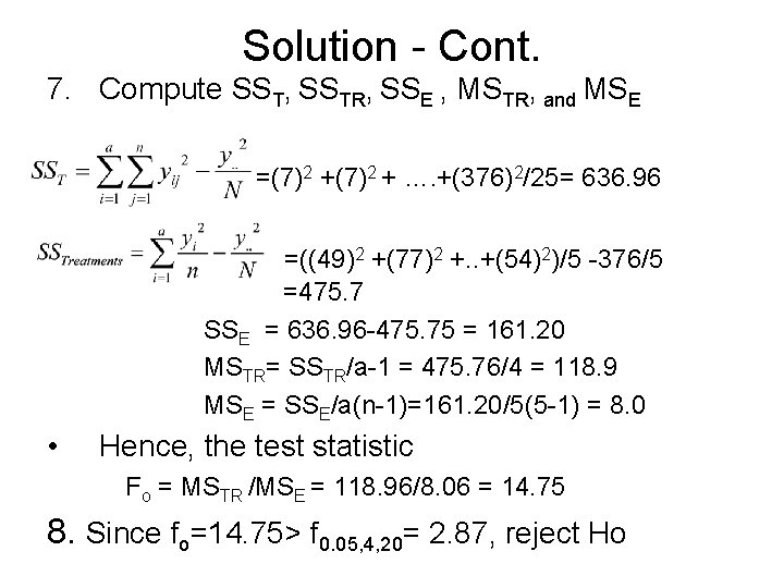
Solution - Cont. 7. Compute SST, SSTR, SSE , MSTR, and MSE =(7)2 + …. +(376)2/25= 636. 96 =((49)2 +(77)2 +. . +(54)2)/5 -376/5 =475. 7 SSE = 636. 96 -475. 75 = 161. 20 MSTR= SSTR/a-1 = 475. 76/4 = 118. 9 MSE = SSE/a(n-1)=161. 20/5(5 -1) = 8. 0 • Hence, the test statistic Fo = MSTR /MSE = 118. 96/8. 06 = 14. 75 8. Since fo=14. 75> f 0. 05, 4, 20= 2. 87, reject Ho

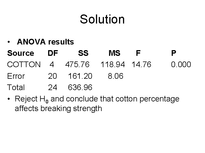
Solution • ANOVA results Source DF SS MS F P COTTON 4 475. 76 118. 94 14. 76 0. 000 Error 20 161. 20 8. 06 Total 24 636. 96 • Reject H 0 and conclude that cotton percentage affects breaking strength

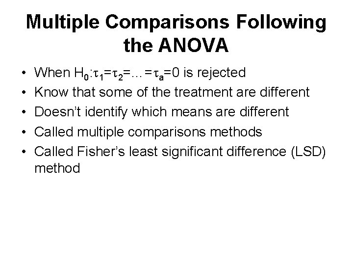
Multiple Comparisons Following the ANOVA • • • When H 0: 1= 2=…= a=0 is rejected Know that some of the treatment are different Doesn’t identify which means are different Called multiple comparisons methods Called Fisher’s least significant difference (LSD) method

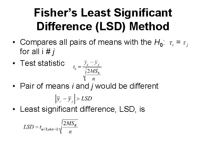
Fisher’s Least Significant Difference (LSD) Method • Compares all pairs of means with the H 0: for all i # j • Test statistic • Pair of means i and j would be different • Least significant difference, LSD, is =

Example • Use Fisher’s LSD method with α = 0. 05 test to analyze the means of five different levels of cotton percentage content in the previous example • Recall H 0 was rejected and concluded that cotton percentage affects the breaking strength • Apply the Fisher’s LSD method to determine which treatment means are different

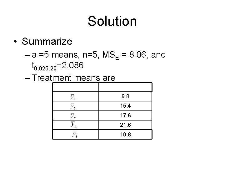
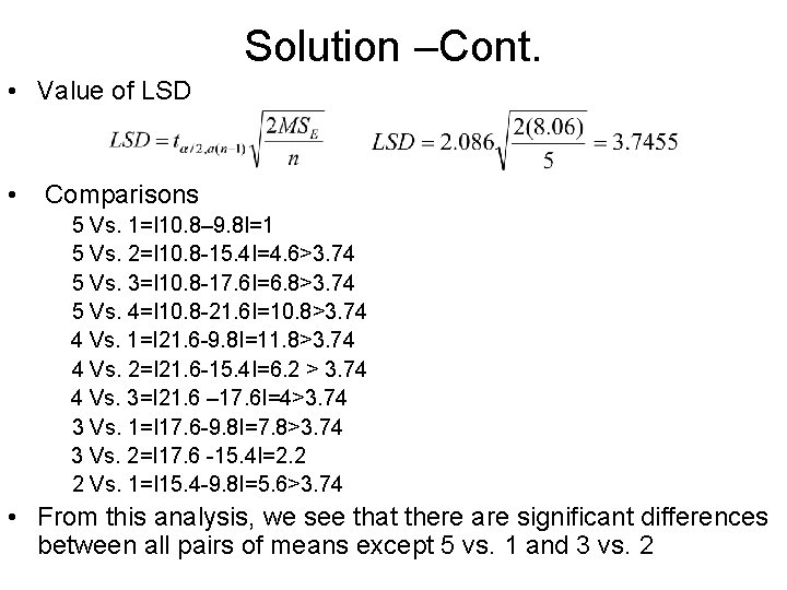
Solution • Summarize – a =5 means, n=5, MSE = 8. 06, and t 0. 025, 20=2. 086 – Treatment means are 9. 8 15. 4 17. 6 21. 6 10. 8

Solution –Cont. • Value of LSD • Comparisons 5 Vs. 1=I 10. 8– 9. 8 I=1 5 Vs. 2=I 10. 8 -15. 4 I=4. 6>3. 74 5 Vs. 3=I 10. 8 -17. 6 I=6. 8>3. 74 5 Vs. 4=I 10. 8 -21. 6 I=10. 8>3. 74 4 Vs. 1=I 21. 6 -9. 8 I=11. 8>3. 74 4 Vs. 2=I 21. 6 -15. 4 I=6. 2 > 3. 74 4 Vs. 3=I 21. 6 – 17. 6 I=4>3. 74 3 Vs. 1=I 17. 6 -9. 8 I=7. 8>3. 74 3 Vs. 2=I 17. 6 -15. 4 I=2. 2 2 Vs. 1=I 15. 4 -9. 8 I=5. 6>3. 74 • From this analysis, we see that there are significant differences between all pairs of means except 5 vs. 1 and 3 vs. 2

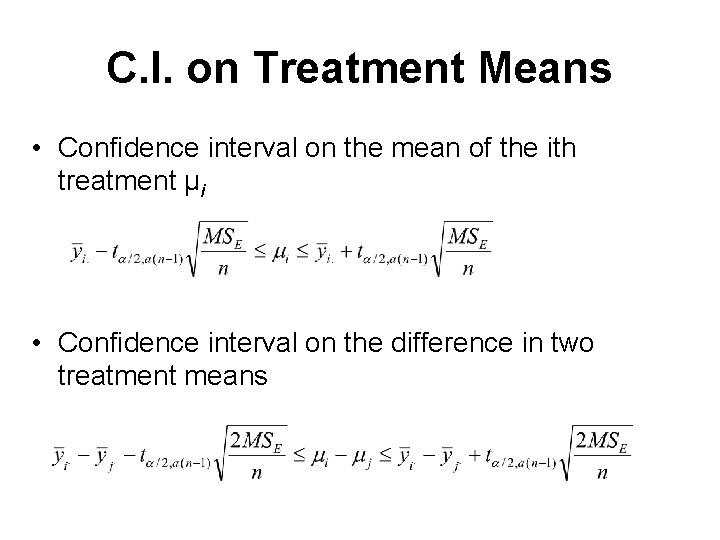
C. I. on Treatment Means • Confidence interval on the mean of the ith treatment µi • Confidence interval on the difference in two treatment means

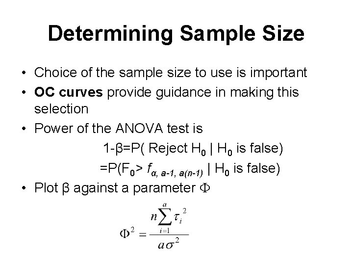
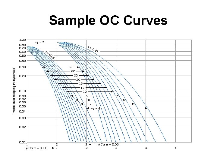
Determining Sample Size • Choice of the sample size to use is important • OC curves provide guidance in making this selection • Power of the ANOVA test is 1 -β=P( Reject H 0 | H 0 is false) =P(F 0> fα, a-1, a(n-1) | H 0 is false) • Plot β against a parameter

Sample OC Curves

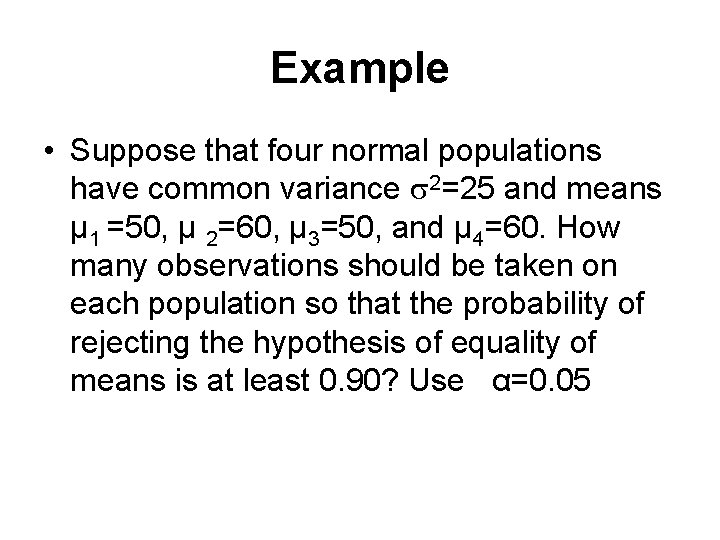
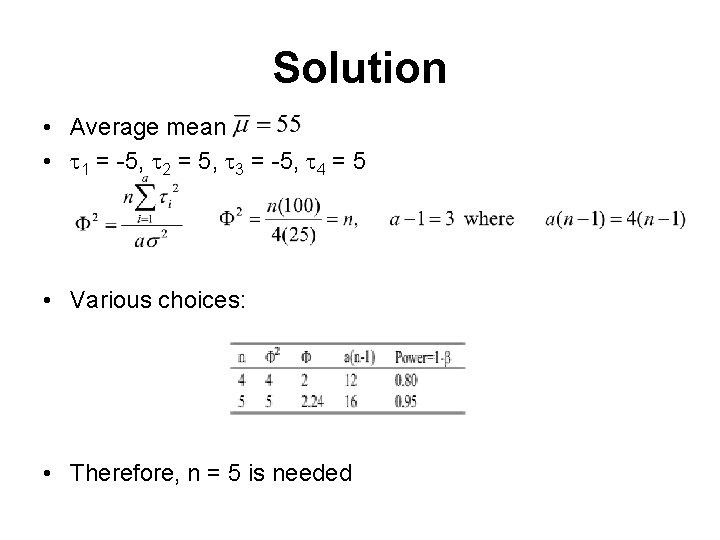
Example • Suppose that four normal populations have common variance 2=25 and means µ 1 =50, µ 2=60, µ 3=50, and µ 4=60. How many observations should be taken on each population so that the probability of rejecting the hypothesis of equality of means is at least 0. 90? Use α=0. 05

Solution • Average mean • 1 = -5, 2 = 5, 3 = -5, 4 = 5 • Various choices: • Therefore, n = 5 is needed

The Random-effects Model • A large number of possible levels • Experimenter randomly selects a of these levels from the population of factor levels – Called random-effect model • Valid for the entire population of factor levels

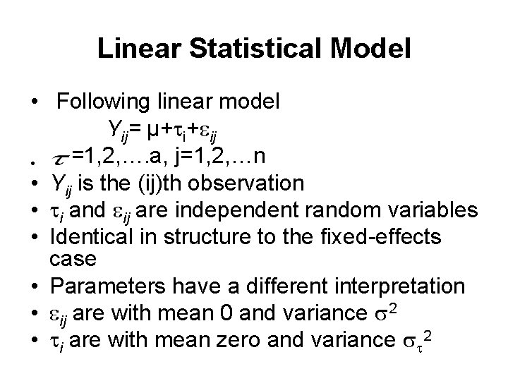
Linear Statistical Model • Following linear model Yij= µ+ i+ ij =1, 2, …. a, j=1, 2, …n • • Yij is the (ij)th observation • i and ij are independent random variables • Identical in structure to the fixed-effects case • Parameters have a different interpretation • ij are with mean 0 and variance 2 • i are with mean zero and variance 2

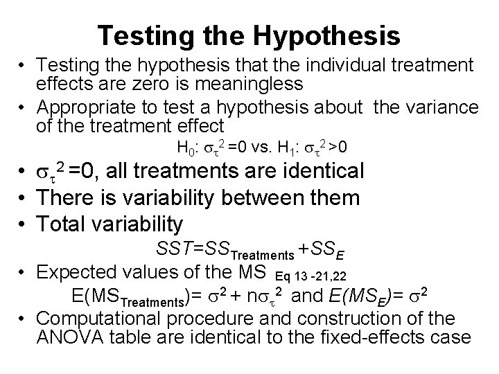
Testing the Hypothesis • Testing the hypothesis that the individual treatment effects are zero is meaningless • Appropriate to test a hypothesis about the variance of the treatment effect H 0: 2 =0 vs. H 1: 2 >0 • 2 =0, all treatments are identical • There is variability between them • Total variability SST=SSTreatments +SSE • Expected values of the MS Eq 13 -21, 22 E(MSTreatments)= 2 + n 2 and E(MSE)= 2 • Computational procedure and construction of the ANOVA table are identical to the fixed-effects case

Randomized Complete Block Design • Desired to design an experiment so that the variability arising from a nuisance factor can be controlled • Recall about the paired t-test • When all experimental runs cannot be made under homogeneous conditions • See the paired t-test as a method for reducing the noise in the experiment by blocking out a nuisance factor effect • Randomized block design can be viewed as an extension of the paired t-test • Factor of interest has more than two levels • More than two treatments must be compared

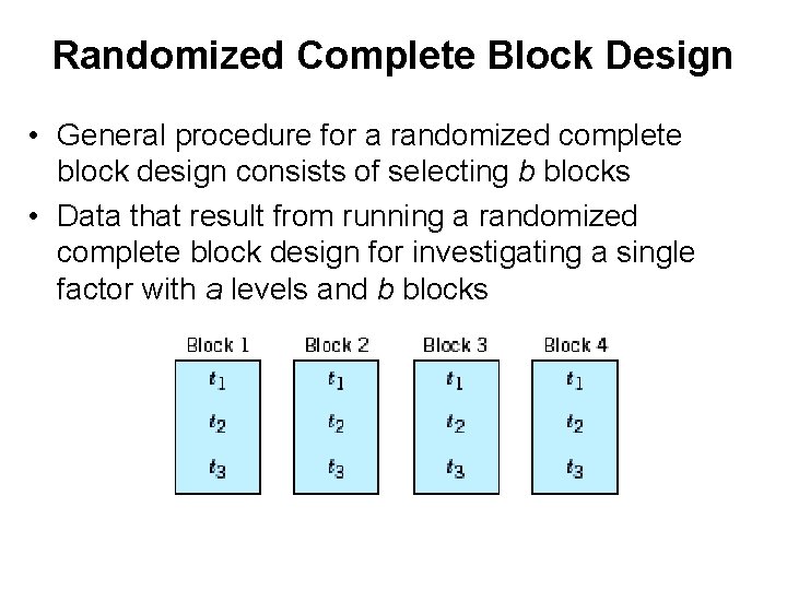
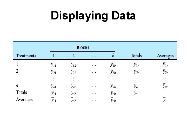
Randomized Complete Block Design • General procedure for a randomized complete block design consists of selecting b blocks • Data that result from running a randomized complete block design for investigating a single factor with a levels and b blocks

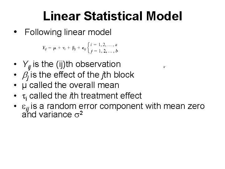
Linear Statistical Model • Following linear model • • • Yij is the (ij)th observation j is the effect of the jth block µ called the overall mean i called the ith treatment effect ij is a random error component with mean zero and variance 2

Hypothesis Testing • • Interested in testing the equality of the a treatment means 1, 2 …. . a Equivalent H 0: 1= 2=…= a=0 H 1: a#0 for at least one i • If the null hypothesis is true, changing the levels of the factor has no effect on the mean response

Displaying Data

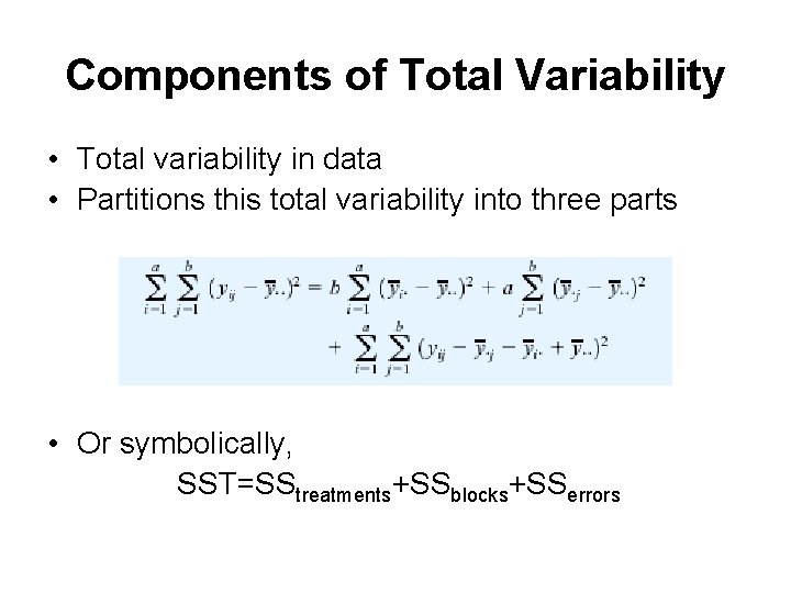
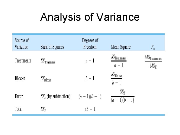
Components of Total Variability • Total variability in data • Partitions this total variability into three parts • Or symbolically, SST=SStreatments+SSblocks+SSerrors

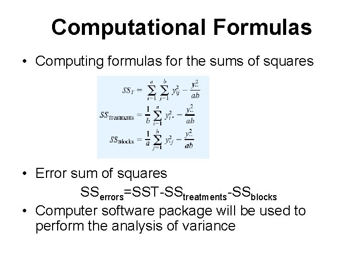
Computational Formulas • Computing formulas for the sums of squares • Error sum of squares SSerrors=SST-SStreatments-SSblocks • Computer software package will be used to perform the analysis of variance

Analysis of Variance

Next Agenda • Ends our discussion with the analysis of variance when there are more then two levels of a single factor • In the next chapter, we will show to design and analyze experiments with several factors with more than two levels