Experiments Statistics Experiment Design Playtesting Experiments dont have

Experiments & Statistics

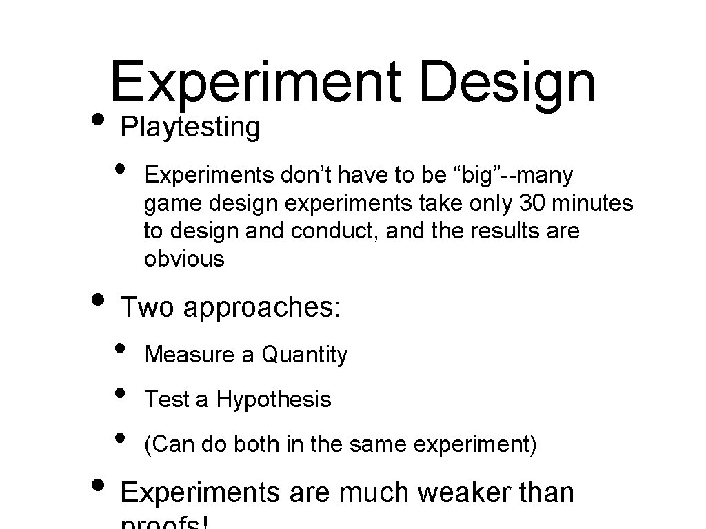
Experiment Design • Playtesting • Experiments don’t have to be “big”--many game design experiments take only 30 minutes to design and conduct, and the results are obvious • Two approaches: • • • Measure a Quantity Test a Hypothesis (Can do both in the same experiment) • Experiments are much weaker than

Control Group • Establish a baseline • Detect any outside factors that might influence the experiment • e. g. , location, testing process itself, temperature, day of week, recent events

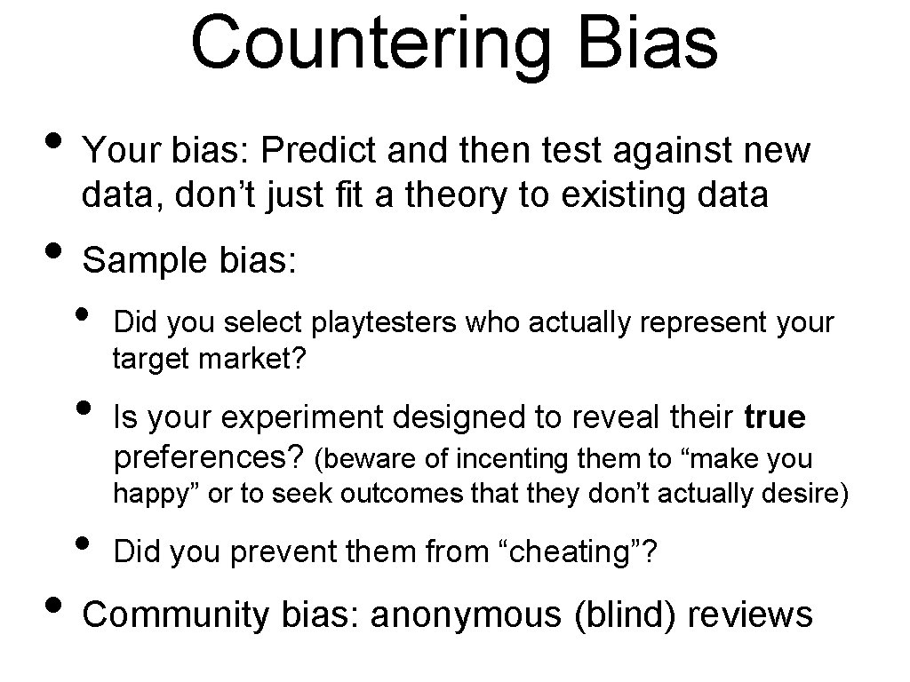
Countering Bias • Your bias: Predict and then test against new data, don’t just fit a theory to existing data • Sample bias: • • Did you select playtesters who actually represent your target market? Is your experiment designed to reveal their true preferences? (beware of incenting them to “make you happy” or to seek outcomes that they don’t actually desire) • Did you prevent them from “cheating”? • Community bias: anonymous (blind) reviews

Measurement (and Statistics)

Example: Measuring Time • Play N turns of a game, measuring the time per turn • We can now predict how long the game will run without further testing, even after we change the rules. • (How large should N be? )

Accuracy vs. Precision • Experiments estimate values; they are never exact • Accuracy is how close your measurement is to the true value (significant digits) • Precision is the number of decimal places in your measurement

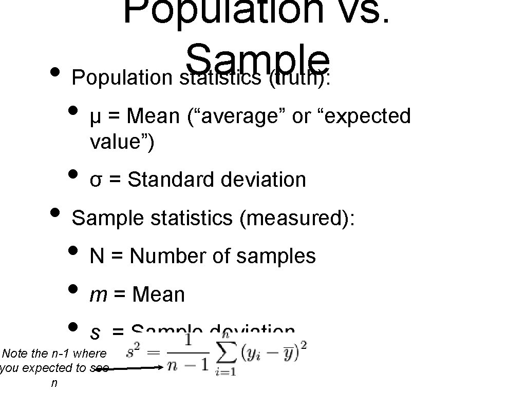
Population vs. Sample • Population statistics (truth): • μ = Mean (“average” or “expected value”) • σ = Standard deviation • Sample statistics (measured): • N = Number of samples • m = Mean • s = Sample deviation Note the n-1 where you expected to see n

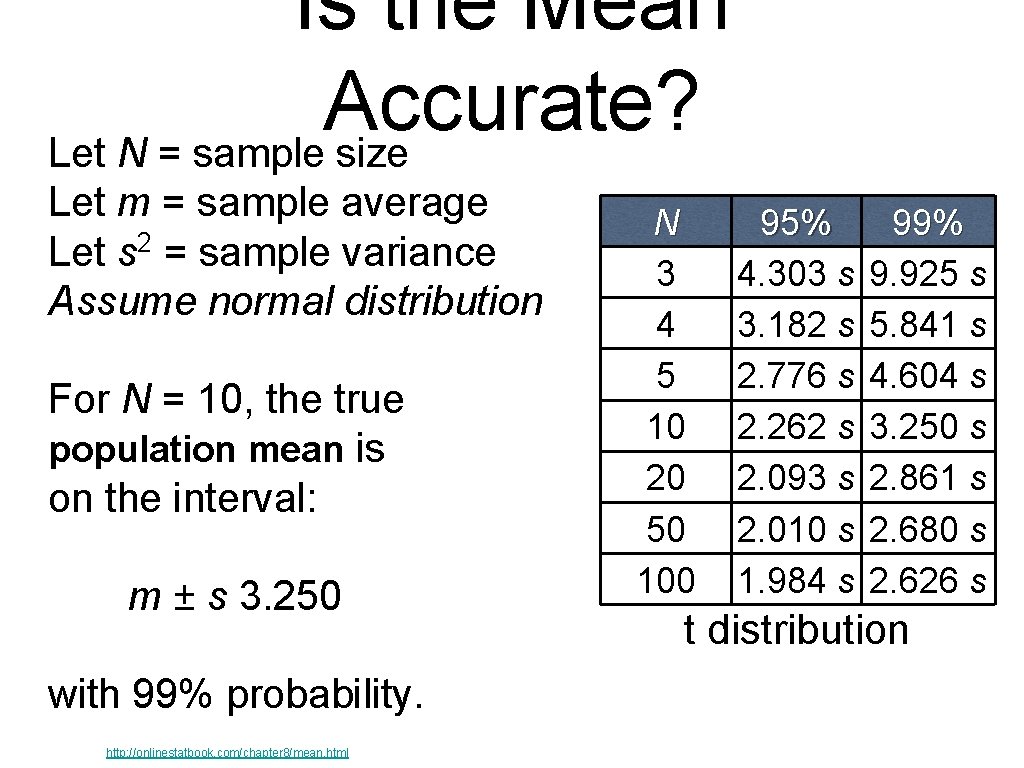
Is the Mean Accurate? Let N = sample size Let m = sample average Let s 2 = sample variance Assume normal distribution For N = 10, the true population mean is on the interval: m ± s 3. 250 with 99% probability. http: //onlinestatbook. com/chapter 8/mean. html N 3 4 5 10 20 50 100 95% 4. 303 s 3. 182 s 2. 776 s 2. 262 s 2. 093 s 2. 010 s 1. 984 s 99% 9. 925 s 5. 841 s 4. 604 s 3. 250 s 2. 861 s 2. 680 s 2. 626 s t distribution

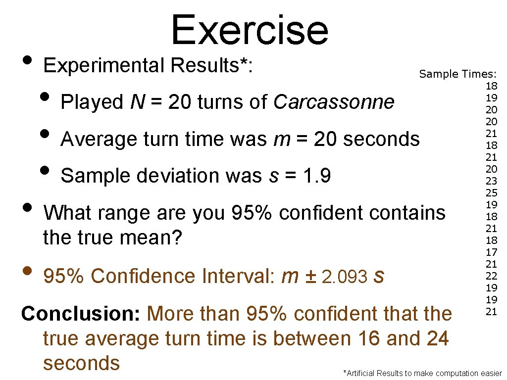
Exercise • Experimental Results*: • Played N = 20 turns of Carcassonne • Average turn time was m = 20 seconds • Sample deviation was s = 1. 9 • What range are you 95% confident contains the true mean? • 95% Confidence Interval: m ± 2. 093 s Sample Times: 18 19 20 20 21 18 21 20 23 25 19 18 21 18 17 21 22 19 19 21 Conclusion: More than 95% confident that the true average turn time is between 16 and 24 seconds *Artificial Results to make computation easier

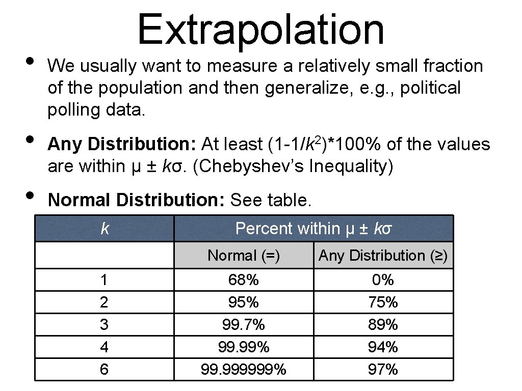
• • • Extrapolation We usually want to measure a relatively small fraction of the population and then generalize, e. g. , political polling data. Any Distribution: At least (1 -1/k 2)*100% of the values are within μ ± kσ. (Chebyshev’s Inequality) Normal Distribution: See table. k 1 2 3 4 6 Percent within μ ± kσ Normal (=) Any Distribution (≥) 68% 95% 99. 7% 99. 999999% 0% 75% 89% 94% 97%

Is the Variance Accurate? • The previous slide assumed that we knew the population variables μ and σ! • We know how to tell if m is accurate. . . • But is s accurate? • Good question. In this class, we’ll just assume that it is. . .

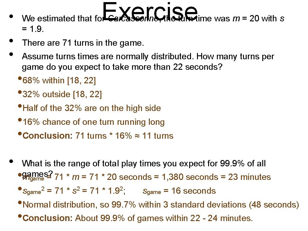
• • • Exercise We estimated that for Carcassonne, the turn time was m = 20 with s = 1. 9. There are 71 turns in the game. Assume turns times are normally distributed. How many turns per game do you expect to take more than 22 seconds? • 68% within [18, 22] • 32% outside [18, 22] • Half of the 32% are on the high side • 16% chance of one turn running long • Conclusion: 71 turns * 16% ≈ 11 turns • What is the range of total play times you expect for 99. 9% of all games? mgame = 71 * m = 71 * 20 seconds = 1, 380 seconds = 23 minutes • • s = 71 * 1. 9 ; s = 16 seconds • Normal distribution, so 99. 7% within 3 standard deviations (48 seconds) • Conclusion: About 99. 9% of games within 22 - 24 minutes. game 2 2 2 game

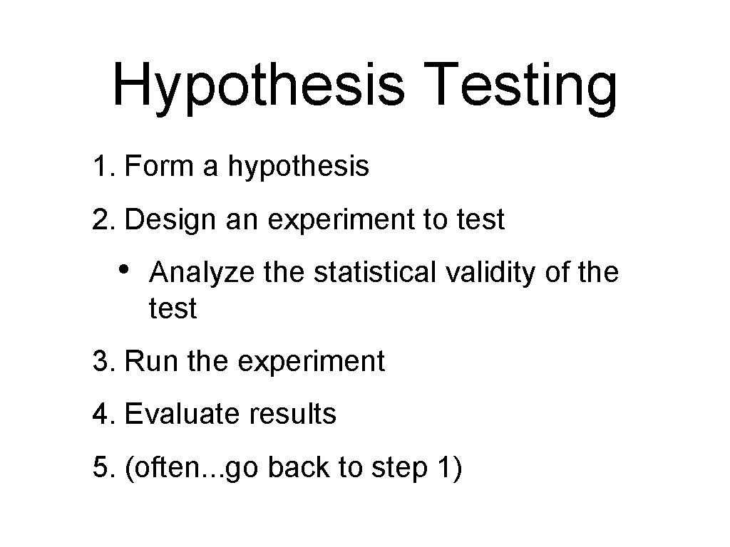
Hypothesis Testing 1. Form a hypothesis 2. Design an experiment to test • Analyze the statistical validity of the test 3. Run the experiment 4. Evaluate results 5. (often. . . go back to step 1)

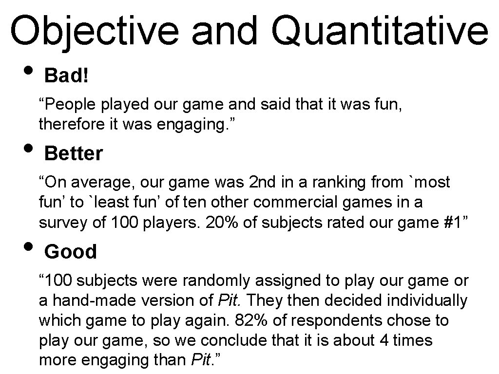
Objective and Quantitative • Bad! “People played our game and said that it was fun, therefore it was engaging. ” • Better “On average, our game was 2 nd in a ranking from `most fun’ to `least fun’ of ten other commercial games in a survey of 100 players. 20% of subjects rated our game #1” • Good “ 100 subjects were randomly assigned to play our game or a hand-made version of Pit. They then decided individually which game to play again. 82% of respondents chose to play our game, so we conclude that it is about 4 times more engaging than Pit. ”

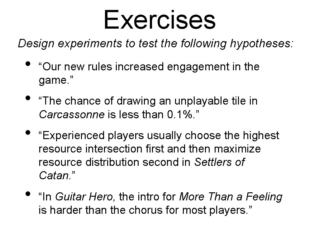
Exercises Design experiments to test the following hypotheses: • • “Our new rules increased engagement in the game. ” “The chance of drawing an unplayable tile in Carcassonne is less than 0. 1%. ” “Experienced players usually choose the highest resource intersection first and then maximize resource distribution second in Settlers of Catan. ” “In Guitar Hero, the intro for More Than a Feeling is harder than the chorus for most players. ”

Exercises Design experiments to test the following hypotheses: • • “Our new rules increased engagement in the game. ” “The chance of drawing an unplayable tile in Carcassonne is less than 0. 1%. ” “Experienced players usually choose the highest resource intersection first and then maximize resource distribution second in Settlers of Catan. ” “In Guitar Hero, the intro for More Than a Feeling is harder than the chorus for most players. ”