Topic 3 Ch 8 Index Models A singlefactor

Topic 3 (Ch. 8) Index Models • A single-factor security market • The single-index model • Estimating the single-index model 1

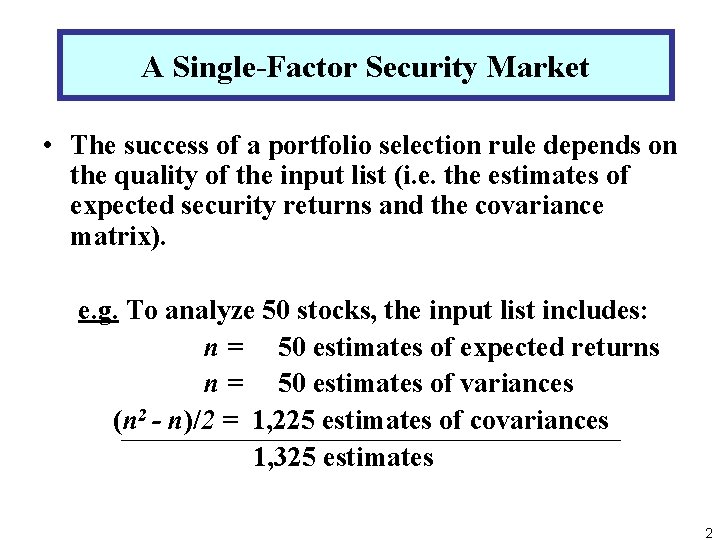
A Single-Factor Security Market • The success of a portfolio selection rule depends on the quality of the input list (i. e. the estimates of expected security returns and the covariance matrix). e. g. To analyze 50 stocks, the input list includes: n = 50 estimates of expected returns n = 50 estimates of variances (n 2 - n)/2 = 1, 225 estimates of covariances 1, 325 estimates 2

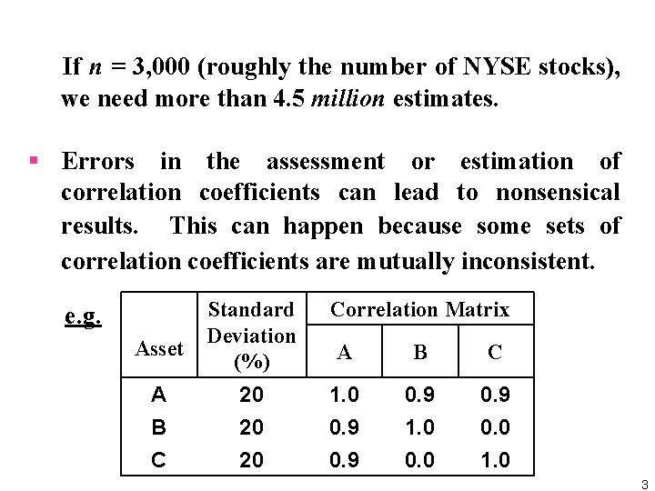
If n = 3, 000 (roughly the number of NYSE stocks), we need more than 4. 5 million estimates. § Errors in the assessment or estimation of correlation coefficients can lead to nonsensical results. This can happen because some sets of correlation coefficients are mutually inconsistent. e. g. Asset Standard Deviation (%) Correlation Matrix A B C A 20 1. 0 0. 9 B 20 0. 9 1. 0 0. 0 C 20 0. 9 0. 0 1. 0 3

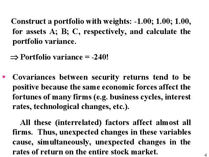
Construct a portfolio with weights: -1. 00; 1. 00, for assets A; B; C, respectively, and calculate the portfolio variance. Portfolio variance = -240! § Covariances between security returns tend to be positive because the same economic forces affect the fortunes of many firms (e. g. business cycles, interest rates, technological changes, etc. ). All these (interrelated) factors affect almost all firms. Thus, unexpected changes in these variables cause, simultaneously, unexpected changes in the rates of return on the entire stock market. 4

• Suppose that we summarize all relevant economic factors by one macroeconomic indicator and assume that it moves the security market as a whole. We further assume that, beyond this common effect, all remaining uncertainty in stock returns is firm specific (i. e. there is no other source of correlation between securities). Firm-specific events would include new inventions, deaths of key employees, and other factors that affect the fortune of the individual firm without affecting the broad economy in a measurable way. 5

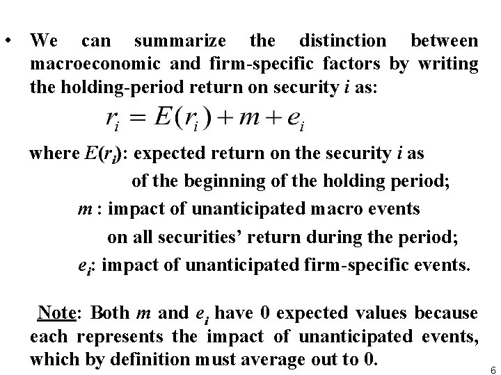
• We can summarize the distinction between macroeconomic and firm-specific factors by writing the holding-period return on security i as: where E(ri): expected return on the security i as of the beginning of the holding period; m : impact of unanticipated macro events on all securities’ return during the period; ei: impact of unanticipated firm-specific events. Note: Both m and ei have 0 expected values because each represents the impact of unanticipated events, which by definition must average out to 0. 6

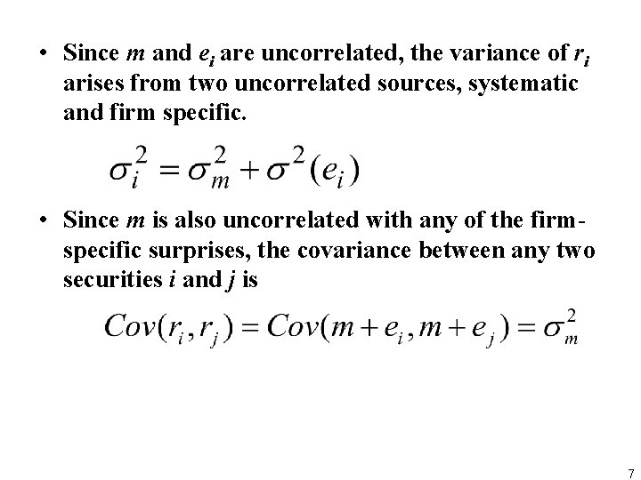
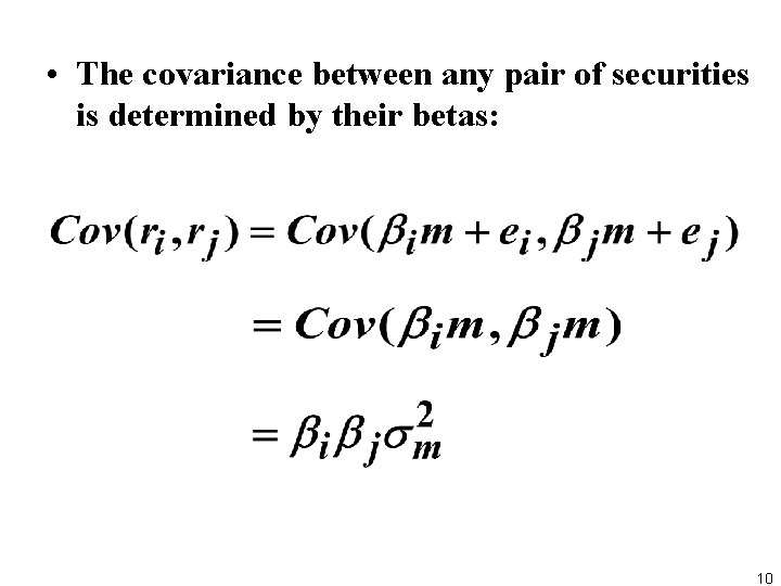
• Since m and ei are uncorrelated, the variance of ri arises from two uncorrelated sources, systematic and firm specific. • Since m is also uncorrelated with any of the firmspecific surprises, the covariance between any two securities i and j is 7

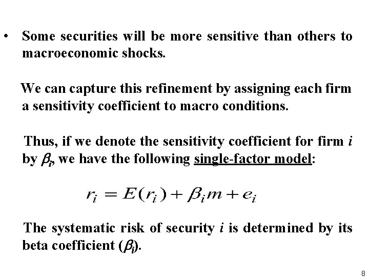
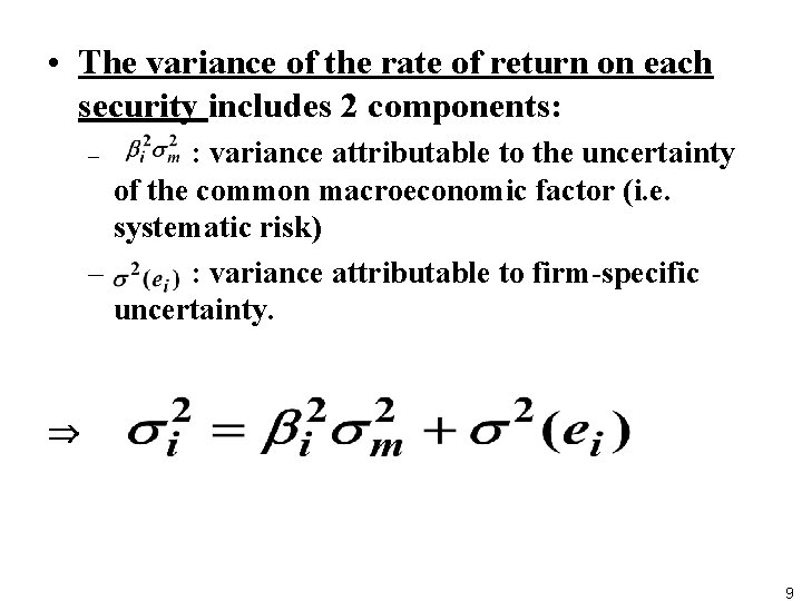
• Some securities will be more sensitive than others to macroeconomic shocks. We can capture this refinement by assigning each firm a sensitivity coefficient to macro conditions. Thus, if we denote the sensitivity coefficient for firm i by i, we have the following single-factor model: The systematic risk of security i is determined by its beta coefficient ( i). 8

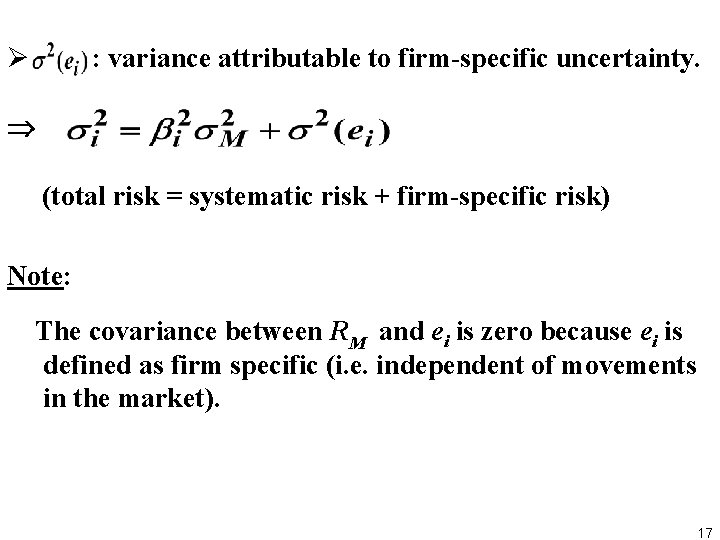
• The variance of the rate of return on each security includes 2 components: : variance attributable to the uncertainty of the common macroeconomic factor (i. e. systematic risk) – : variance attributable to firm-specific uncertainty. – 9

• The covariance between any pair of securities is determined by their betas: 10

The Single-Index Model • To make the single-factor model operational, we use the rate of return on a broad index of securities (such as S&P 500) as a proxy for the common macroeconomic factor. This approach leads to an equation similar to the single-factor model, which is called the single-index model, because it uses the market index to proxy for the common factor. 11

The regression equation of the single-index model • Denote the market index by M, with excess return of RM = r. M - rf and standard deviation of σM. • Excess return of a security: R i = r i – rf 12

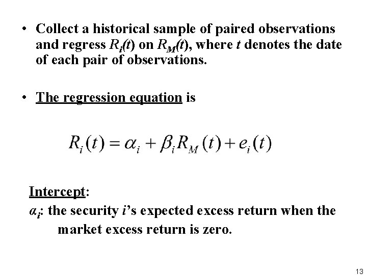
• Collect a historical sample of paired observations and regress Ri(t) on RM(t), where t denotes the date of each pair of observations. • The regression equation is Intercept: αi: the security i’s expected excess return when the market excess return is zero. 13

Slope coefficient: βi: the security i’s sensitivity to the market index. For every + (or -) 1% change in the market excess return, the excess return on the security will change by + (or -)βi%. Residual: ei is the zero-mean, firm specific surprise in the security return in time t. 14

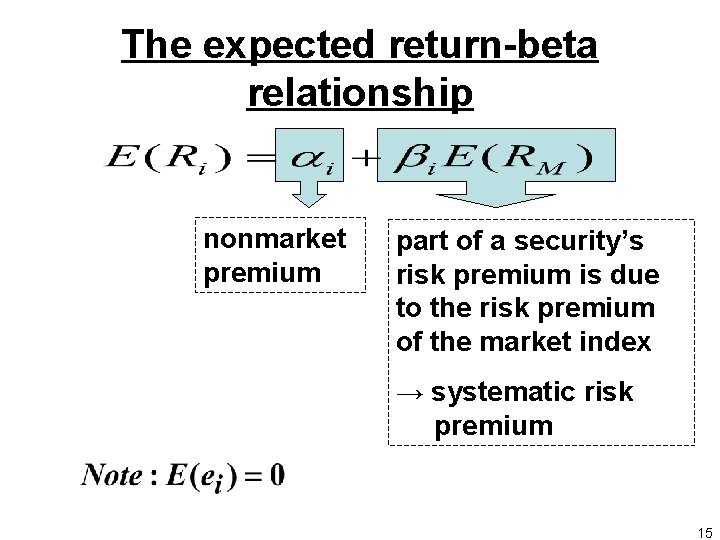
The expected return-beta relationship nonmarket premium part of a security’s risk premium is due to the risk premium of the market index → systematic risk premium 15

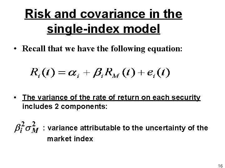
Risk and covariance in the single-index model • Recall that we have the following equation: • The variance of the rate of return on each security includes 2 components: : variance attributable to the uncertainty of the market index 16

Ø : variance attributable to firm-specific uncertainty. (total risk = systematic risk + firm-specific risk) Note: The covariance between RM and ei is zero because ei is defined as firm specific (i. e. independent of movements in the market). 17

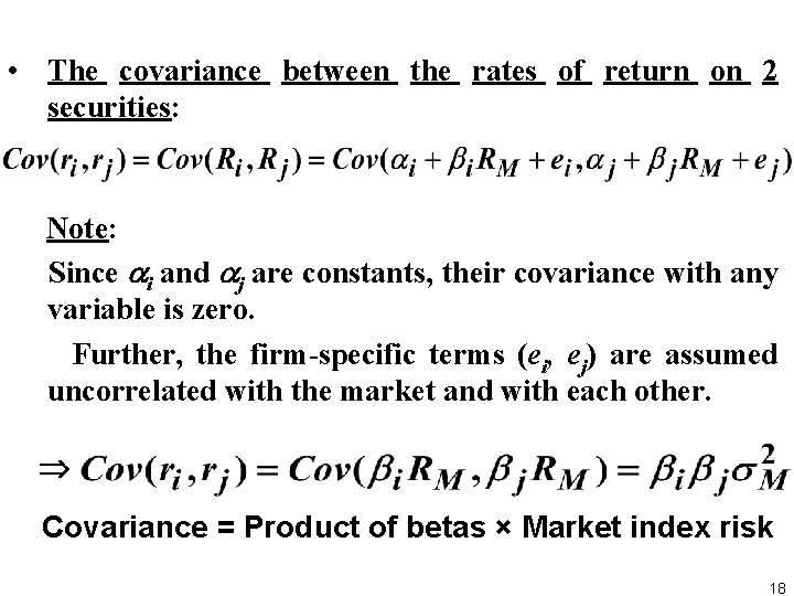
• The covariance between the rates of return on 2 securities: Note: Since i and j are constants, their covariance with any variable is zero. Further, the firm-specific terms (ei, ej) are assumed uncorrelated with the market and with each other. Covariance = Product of betas × Market index risk 18

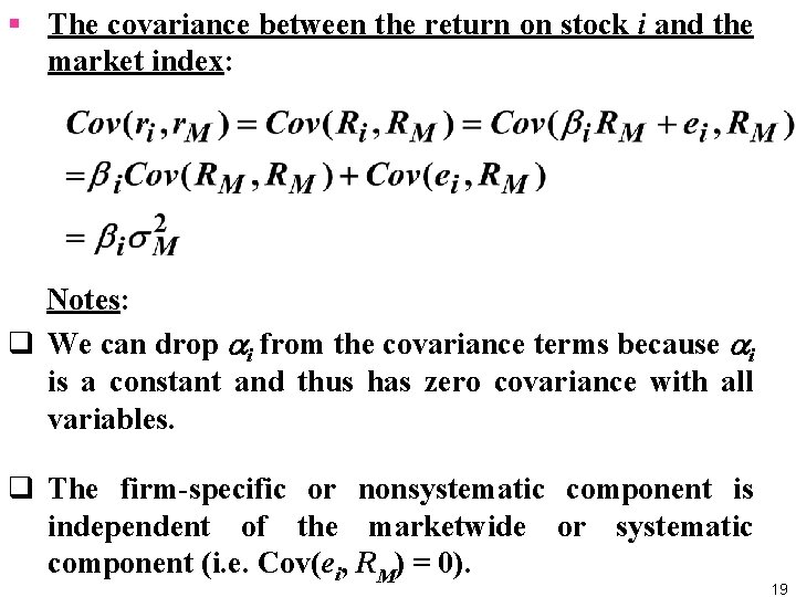
§ The covariance between the return on stock i and the market index: Notes: q We can drop i from the covariance terms because i is a constant and thus has zero covariance with all variables. q The firm-specific or nonsystematic component is independent of the marketwide or systematic component (i. e. Cov(ei, RM) = 0). 19

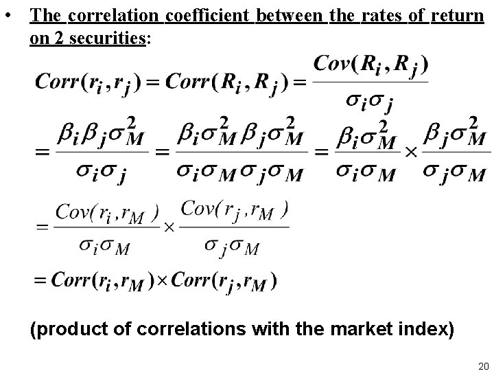
• The correlation coefficient between the rates of return on 2 securities: (product of correlations with the market index) 20

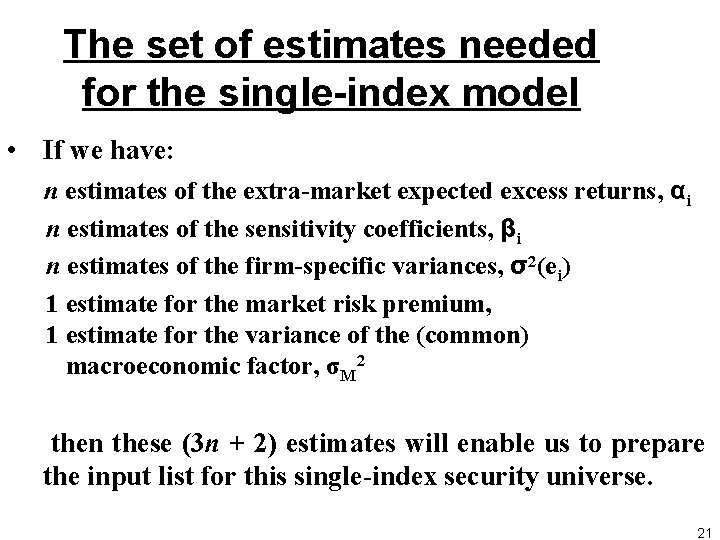
The set of estimates needed for the single-index model • If we have: n estimates of the extra-market expected excess returns, αi n estimates of the sensitivity coefficients, βi n estimates of the firm-specific variances, σ2(ei) 1 estimate for the market risk premium, 1 estimate for the variance of the (common) macroeconomic factor, σM 2 then these (3 n + 2) estimates will enable us to prepare the input list for this single-index security universe. 21

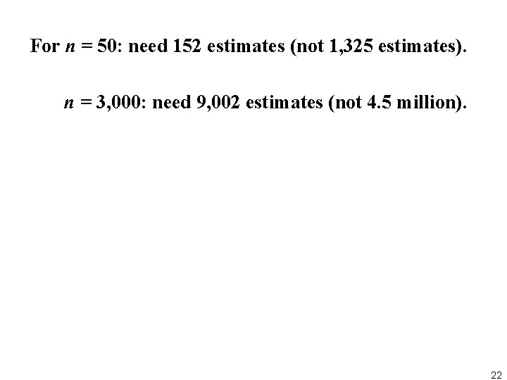
For n = 50: need 152 estimates (not 1, 325 estimates). n = 3, 000: need 9, 002 estimates (not 4. 5 million). 22

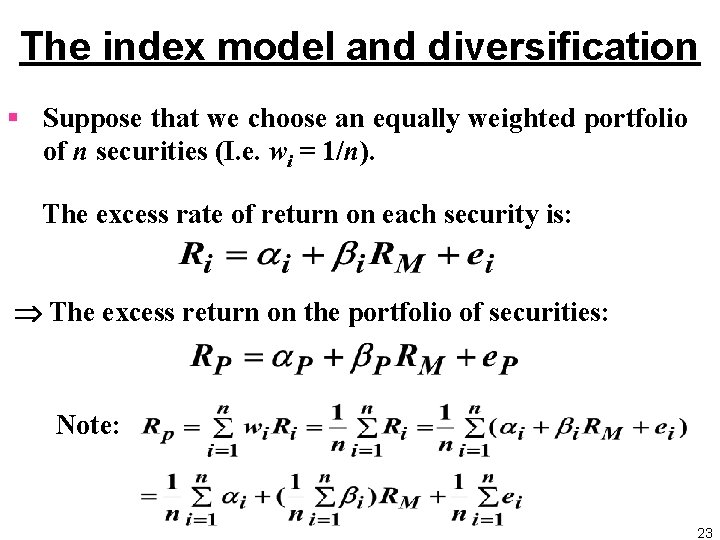
The index model and diversification § Suppose that we choose an equally weighted portfolio of n securities (I. e. wi = 1/n). The excess rate of return on each security is: The excess return on the portfolio of securities: Note: 23

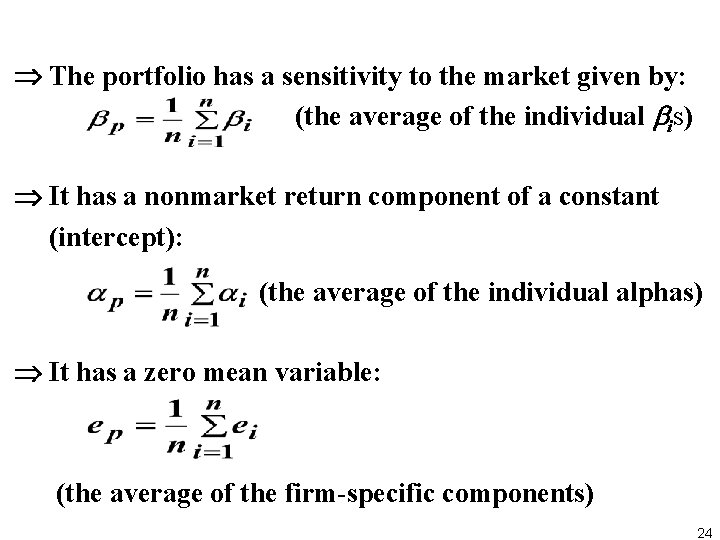
The portfolio has a sensitivity to the market given by: (the average of the individual is) It has a nonmarket return component of a constant (intercept): (the average of the individual alphas) It has a zero mean variable: (the average of the firm-specific components) 24

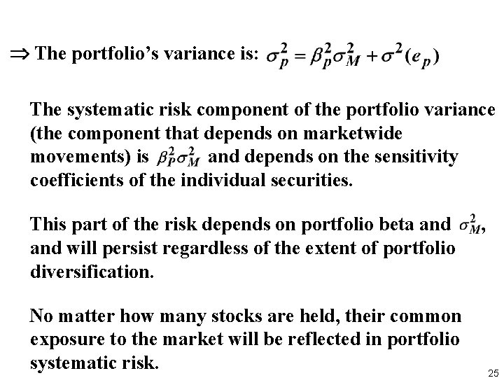
The portfolio’s variance is: The systematic risk component of the portfolio variance (the component that depends on marketwide movements) is and depends on the sensitivity coefficients of the individual securities. This part of the risk depends on portfolio beta and will persist regardless of the extent of portfolio diversification. No matter how many stocks are held, their common exposure to the market will be reflected in portfolio systematic risk. , 25

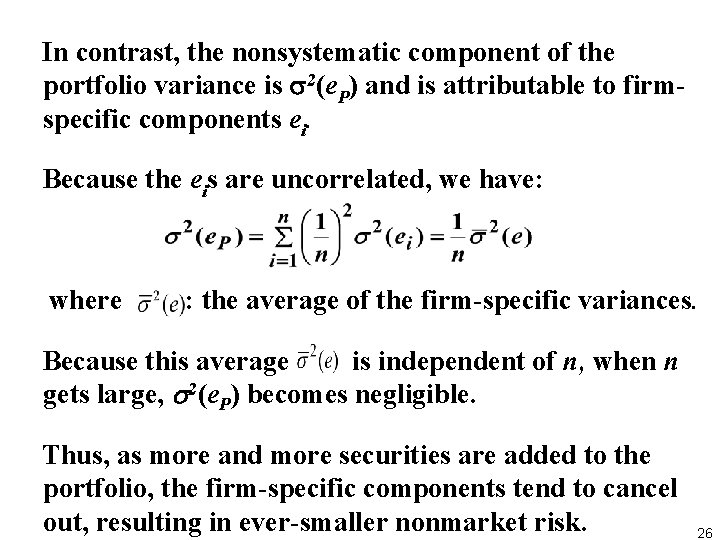
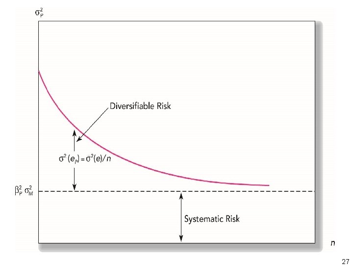
In contrast, the nonsystematic component of the portfolio variance is 2(e. P) and is attributable to firmspecific components ei. Because the eis are uncorrelated, we have: where : the average of the firm-specific variances. Because this average is independent of n, when n gets large, 2(e. P) becomes negligible. Thus, as more and more securities are added to the portfolio, the firm-specific components tend to cancel out, resulting in ever-smaller nonmarket risk. 26

27

Summary: As more and more securities are combined into a portfolio, the portfolio variance decreases because of the diversification of firm-specific risk. However, the power of diversification is limited. Even for very large n, part of the risk remains because of the exposure of virtually all assets to the common, or market, factor. Therefore, this systematic risk is said to be nondiversifiable. 28

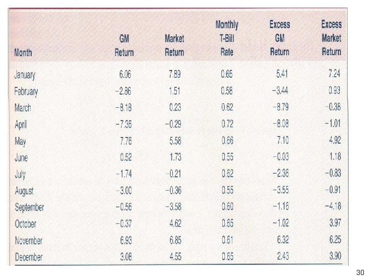
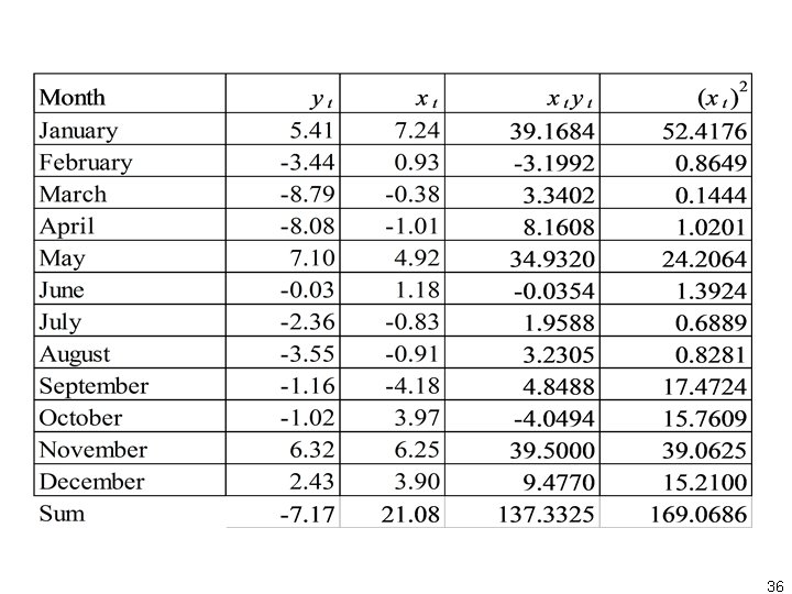
Estimating the Single-Index Model § The single-index model suggests how we might go about actually measuring market and firm-specific risk. Suppose that we observe the excess return on the market index and a specific asset over a number of holding periods. We use as an example monthly excess returns on the S&P 500 index and GM stock for a one-year period. 29

30

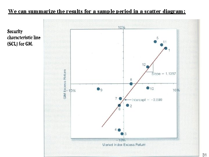
We can summarize the results for a sample period in a scatter diagram: 31

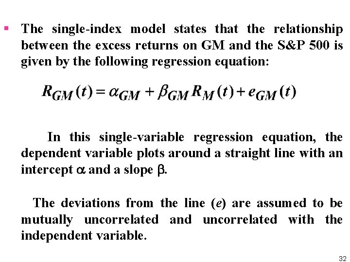
§ The single-index model states that the relationship between the excess returns on GM and the S&P 500 is given by the following regression equation: In this single-variable regression equation, the dependent variable plots around a straight line with an intercept and a slope . The deviations from the line (e) are assumed to be mutually uncorrelated and uncorrelated with the independent variable. 32

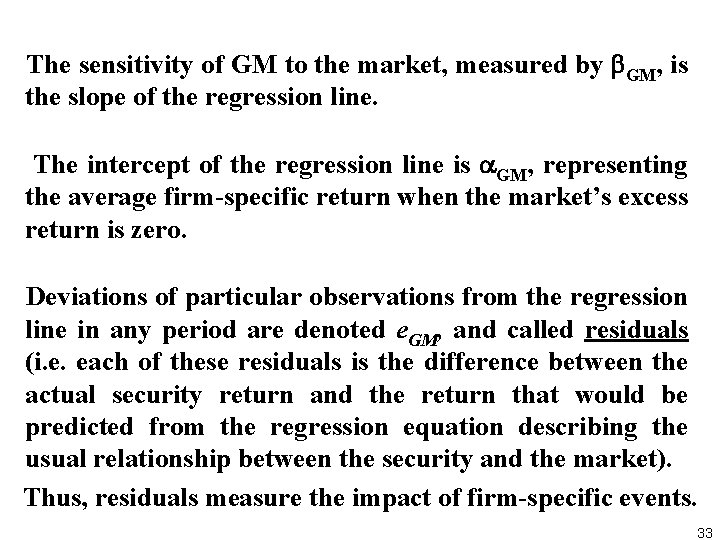
The sensitivity of GM to the market, measured by GM, is the slope of the regression line. The intercept of the regression line is GM, representing the average firm-specific return when the market’s excess return is zero. Deviations of particular observations from the regression line in any period are denoted e. GM, and called residuals (i. e. each of these residuals is the difference between the actual security return and the return that would be predicted from the regression equation describing the usual relationship between the security and the market). Thus, residuals measure the impact of firm-specific events. 33

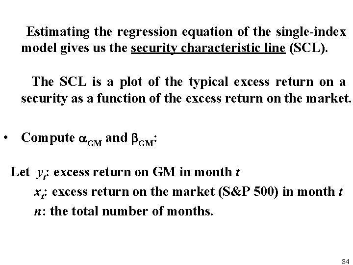
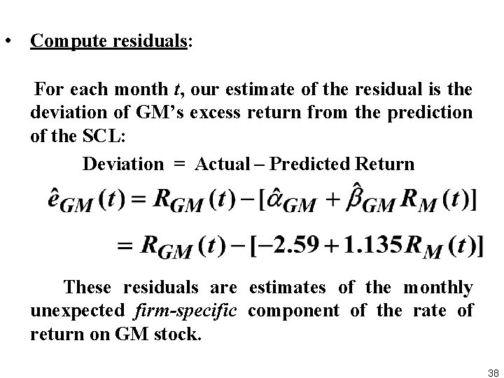
Estimating the regression equation of the single-index model gives us the security characteristic line (SCL). The SCL is a plot of the typical excess return on a security as a function of the excess return on the market. • Compute GM and GM: Let yt: excess return on GM in month t xt: excess return on the market (S&P 500) in month t n: the total number of months. 34

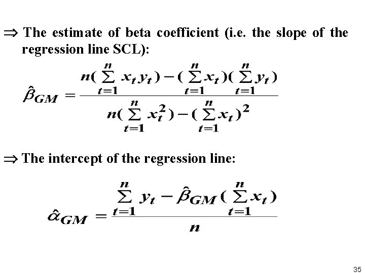
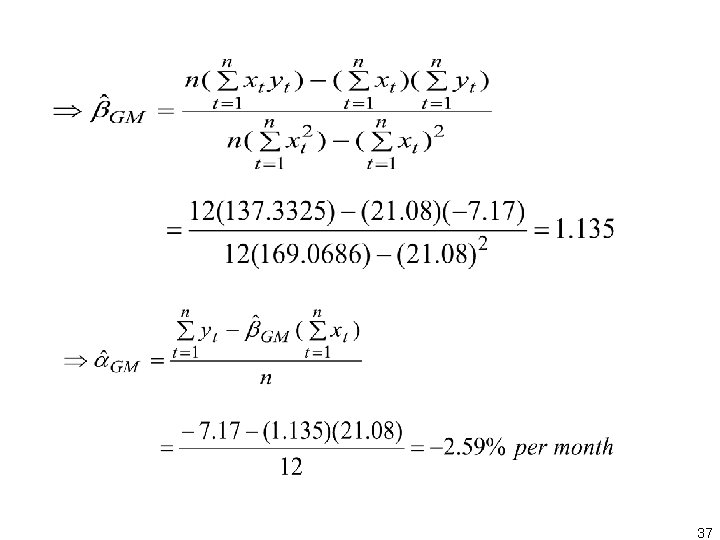
The estimate of beta coefficient (i. e. the slope of the regression line SCL): The intercept of the regression line: 35

36

37

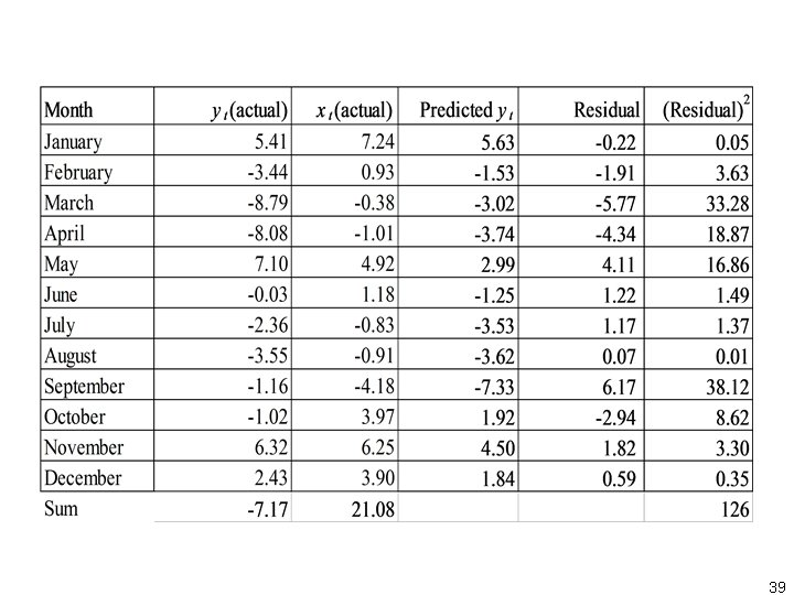
• Compute residuals: For each month t, our estimate of the residual is the deviation of GM’s excess return from the prediction of the SCL: Deviation = Actual – Predicted Return These residuals are estimates of the monthly unexpected firm-specific component of the rate of return on GM stock. 38

39

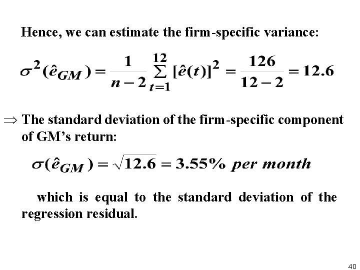
Hence, we can estimate the firm-specific variance: Þ The standard deviation of the firm-specific component of GM’s return: which is equal to the standard deviation of the regression residual. 40

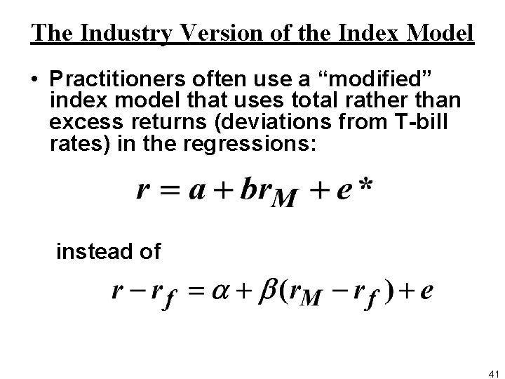
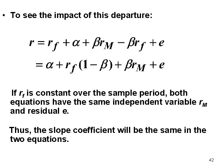
The Industry Version of the Index Model • Practitioners often use a “modified” index model that uses total rather than excess returns (deviations from T-bill rates) in the regressions: instead of 41

• To see the impact of this departure: If rf is constant over the sample period, both equations have the same independent variable r. M and residual e. Thus, the slope coefficient will be the same in the two equations. 42

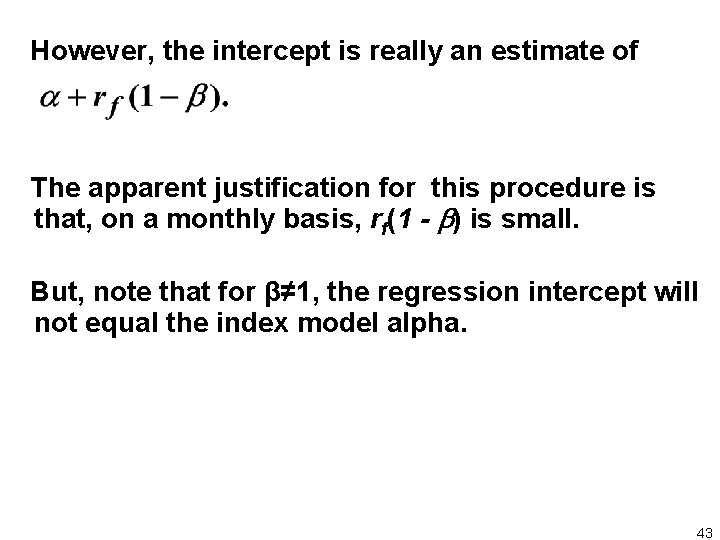
However, the intercept is really an estimate of The apparent justification for this procedure is that, on a monthly basis, rf(1 - ) is small. But, note that for β≠ 1, the regression intercept will not equal the index model alpha. 43

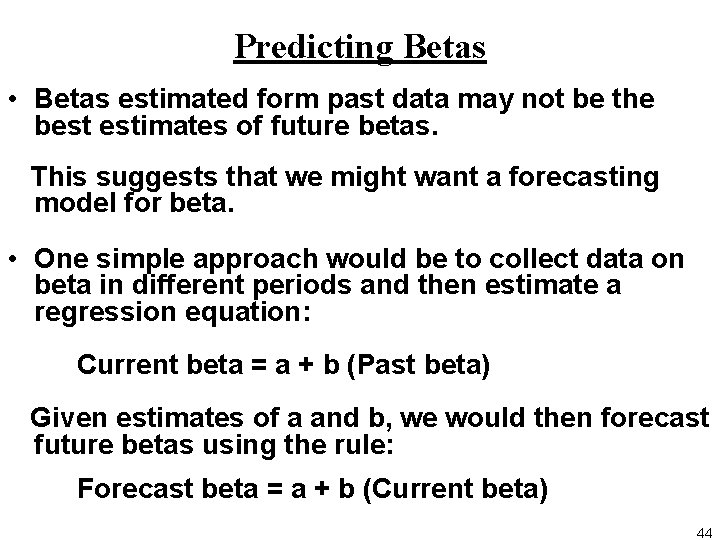
Predicting Betas • Betas estimated form past data may not be the best estimates of future betas. This suggests that we might want a forecasting model for beta. • One simple approach would be to collect data on beta in different periods and then estimate a regression equation: Current beta = a + b (Past beta) Given estimates of a and b, we would then forecast future betas using the rule: Forecast beta = a + b (Current beta) 44

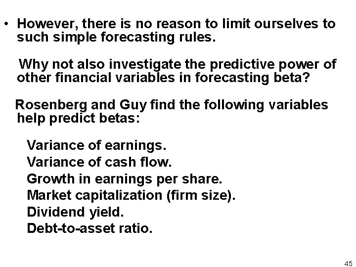
• However, there is no reason to limit ourselves to such simple forecasting rules. Why not also investigate the predictive power of other financial variables in forecasting beta? Rosenberg and Guy find the following variables help predict betas: Variance of earnings. Variance of cash flow. Growth in earnings per share. Market capitalization (firm size). Dividend yield. Debt-to-asset ratio. 45

• Rosenberg and Guy also find that even after controlling for a firm’s financial characteristics, industry group helps to predict beta. 46