Chapter 11 Risk 11 Risk 11 1 Expected

Chapter 11 Risk

11. Risk 11. 1 Expected Utility 11. 2 Attitudes towards Risk 11. 3 Stochastic Dominance◦ 11. 4 Pareto Efficient Risk Sharing 2

Definition Risk is a situation where the uncertainty can be captured by objective probabilities. § Measuring probabilities by: Ø Statistical basis Ø experimental basis Ø analytical basis § The most basic decision theory under risk is the expected utility hypothesis developed by John von Neumann and Oskar Morgenstern § the use of the expected utility hypothesis is widespread in game theory as we will see in Chapter 12 3

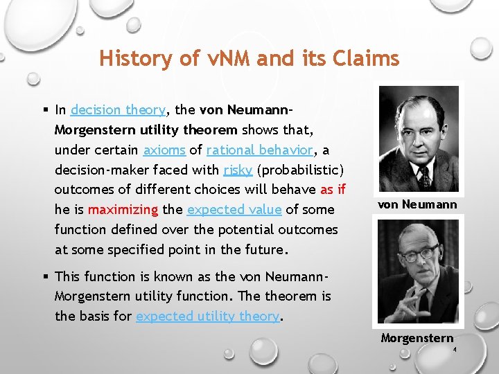
History of v. NM and its Claims § In decision theory, the von Neumann. Morgenstern utility theorem shows that, under certain axioms of rational behavior, a decision-maker faced with risky (probabilistic) outcomes of different choices will behave as if he is maximizing the expected value of some function defined over the potential outcomes at some specified point in the future. von Neumann § This function is known as the von Neumann. Morgenstern utility function. The theorem is the basis for expected utility theory. Morgenstern 4

…History of v. NM and its Claims § In 1947, John von Neumann and Oskar Morgenstern proved that any individual whose preferences satisfied four axioms has a utility function; [1] § They proved that an agent is (VNM-)rational if and only if there exists a real-valued function u defined by possible outcomes such that every preference of the agent is characterized by maximizing the expected value of u, which can then be defined as the agent's VNM-utility (it is unique up to adding a constant and multiplying by a positive scalar). § No claim is made that the agent has a "conscious desire" to maximize u, only that u exists. 5

…History of v. NM and its Claims § Any individual whose preferences violate von Neumann and Morgenstern's axioms would agree to a Dutch book, which is a set of bets that necessarily leads to a loss. § Therefore, it is arguable that any individual who violates the axioms is irrational. § The expected utility hypothesis is that rationality can be modeled as maximizing an expected value, which given theorem, can be summarized as "rationality is VNMrationality". p 6

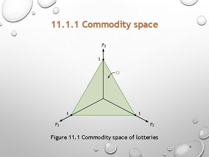
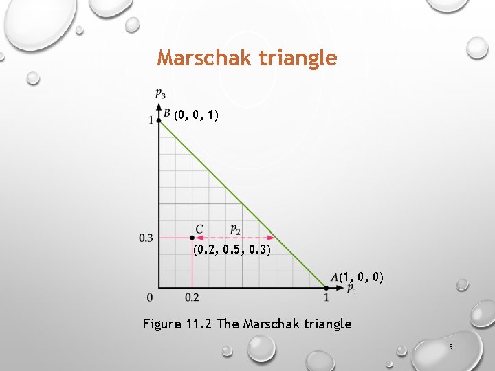
11. 1 Expected Utility § For decision-making under risk the commodity space has to be redefined 11. 1. 1 Commodity space § Prizes: X = {x 1, x 2, x 3} § Lottery: p = (p 1, p 2, p 3) where p 1 + p 2 + p 3 = 1 § The consumer’s decision problem is to choose between different lotteries. § Commodity Space (Δ) is the set of all possible lotteries consisting of any (p 1, p 2, p 3) so long as p 1 + p 2 + p 3 = 1 7

11. 1. 1 Commodity space Figure 11. 1 Commodity space of lotteries 8

Marschak triangle (0, 0, 1) (0. 2, 0. 5, 0. 3) (1, 0, 0) Figure 11. 2 The Marschak triangle 9

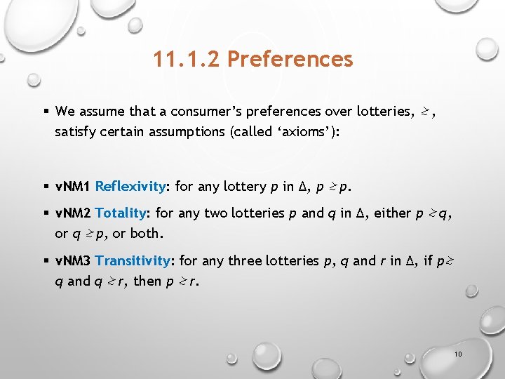
11. 1. 2 Preferences § We assume that a consumer’s preferences over lotteries, ≿ , satisfy certain assumptions (called ‘axioms’): § v. NM 1 Reflexivity: for any lottery p in Δ, p ≿ p. § v. NM 2 Totality: for any two lotteries p and q in Δ, either p ≿ q, or q ≿ p, or both. § v. NM 3 Transitivity: for any three lotteries p, q and r in Δ, if p≿ q and q ≿ r, then p ≿ r. 10

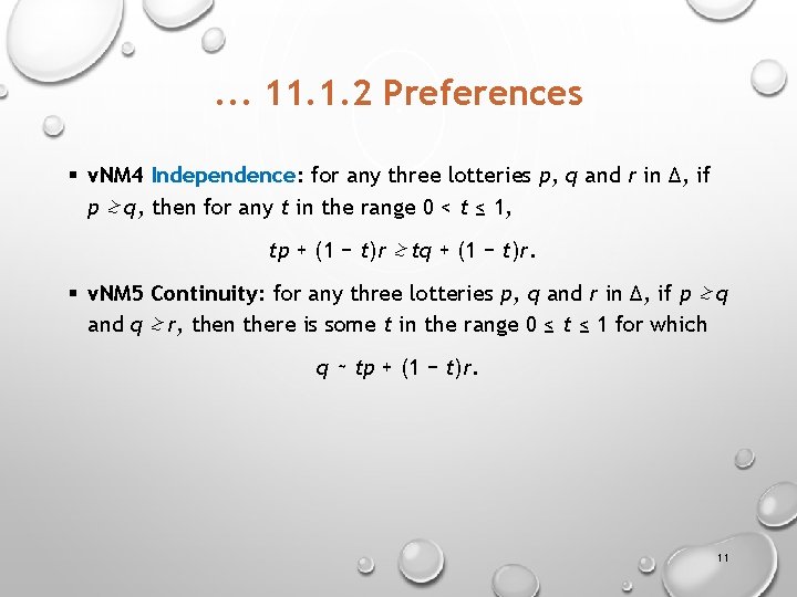
. . . 11. 1. 2 Preferences § v. NM 4 Independence: for any three lotteries p, q and r in Δ, if p ≿ q, then for any t in the range 0 < t ≤ 1, tp + (1 − t)r ≿ tq + (1 − t)r. § v. NM 5 Continuity: for any three lotteries p, q and r in Δ, if p ≿ q and q ≿ r, then there is some t in the range 0 ≤ t ≤ 1 for which q ∼ tp + (1 − t)r. 11

. . . 11. 1. 2 Preferences § The first three axioms should be familiar from Chapter 3 as the requirement for regular preferences § The idea of continuity too is fairly intuitive: if p ≿ q ≿ r, then there is some average of the best and worst lotteries that is indifferent to the one in the middle. § The idea of independence is that the ranking between p and q is independent of any third lottery r when this lottery is averaged with p and q in the same manner. 12

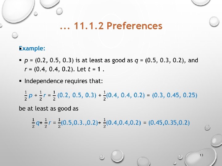
. . . 11. 1. 2 Preferences § 13

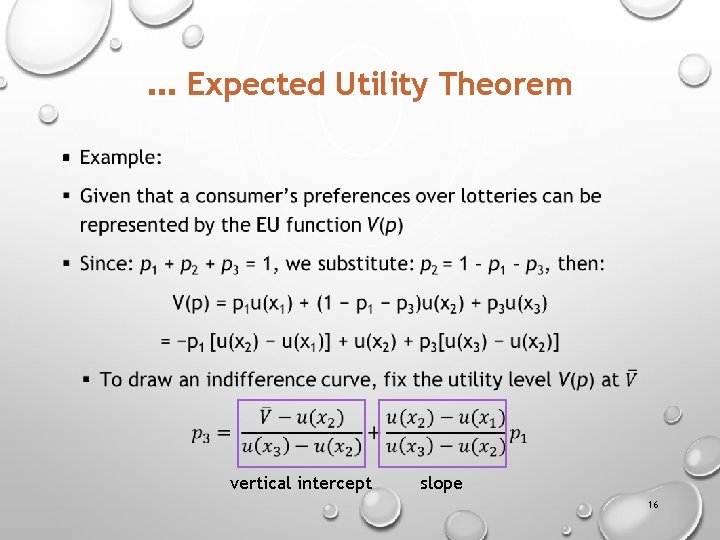
Expected Utility Theorem § If a consumer’s preferences over lotteries satisfy these axioms, then: § (a) there is a von Neumann-Morgenstern (v. NM) utility function u(x) over the set of prizes, X, and § (b) that the consumer’s preferences over lotteries can be represented by an expected utility (EU) function V, where her utility from lottery p is given by V(p) = p 1 u(x 1) + p 2 u(x 2) + p 3 u(x 3) 14

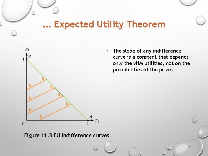
. . . Expected Utility Theorem § FIRST: This theorem holds for any positive monotonic transformation v of the v. NM utility u, so long as v = au + b where a > 0. § SECOND: Because the u(xi) terms are multiplicative constants, the EU function is linear in the probabilities. This implies that the consumer’s preferences over lotteries generate linear indifference curves. 15

. . . Expected Utility Theorem § vertical intercept slope 16

. . . Expected Utility Theorem • The slope of any indifference curve is a constant that depends only the v. NM utilities, not on the probabilities of the prizes Figure 11. 3 EU indifference curves 17

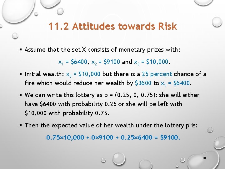
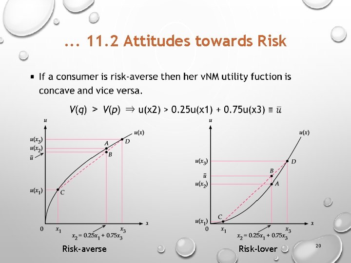
11. 2 Attitudes towards Risk § Assume that the set X consists of monetary prizes with: x 1 = $6400, x 2 = $9100 and x 3 = $10, 000. § Initial wealth: x 3 = $10, 000 but there is a 25 percent chance of a fire which would reduce her wealth by $3600 to x 1 = $6400. § We can write this lottery as p = (0. 25, 0, 0. 75): she will either have $6400 with probability 0. 25 or she will be left with $10, 000 with probability 0. 75. § Then the expected value of her wealth under the lottery p is: 0. 75× 10, 000 + 0× 9100 + 0. 25× 6400 = $9100. 18

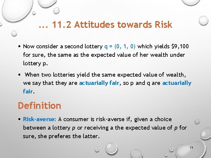
. . . 11. 2 Attitudes towards Risk § Now consider a second lottery q = (0, 1, 0) which yields $9, 100 for sure, the same as the expected value of her wealth under lottery p. § When two lotteries yield the same expected value of wealth, we say that they are actuarially fair, so p and q are actuarially fair. Definition § Risk-averse: A consumer is risk-averse if, given a choice between a lottery p or receiving a the expected value of p for sure, she preferes the latter. 19

. . . 11. 2 Attitudes towards Risk § Risk-averse Risk-lover 20

11. 3 Stochastic Dominance § If one lottery is better than another in some sense, we say that the first stochastically dominates the other § There are two important types of stochastic dominance: Ø first order, and Ø second order 21

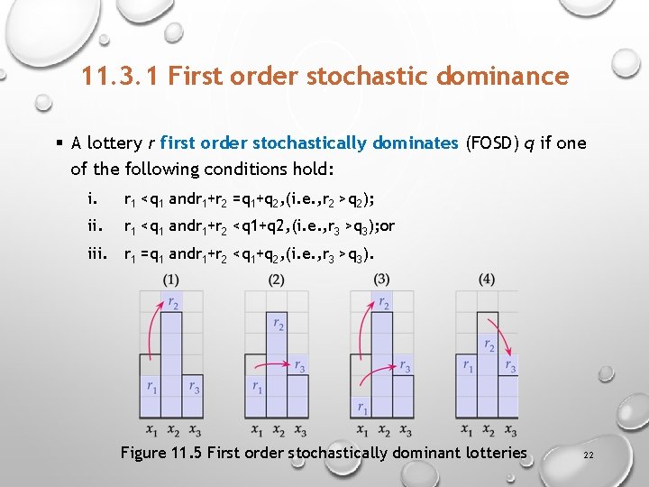
11. 3. 1 First order stochastic dominance § A lottery r first order stochastically dominates (FOSD) q if one of the following conditions hold: i. r 1 <q 1 andr 1+r 2 =q 1+q 2, (i. e. , r 2 >q 2); ii. r 1 <q 1 andr 1+r 2 <q 1+q 2, (i. e. , r 3 >q 3); or iii. r 1 =q 1 andr 1+r 2 <q 1+q 2, (i. e. , r 3 >q 3). Figure 11. 5 First order stochastically dominant lotteries 22

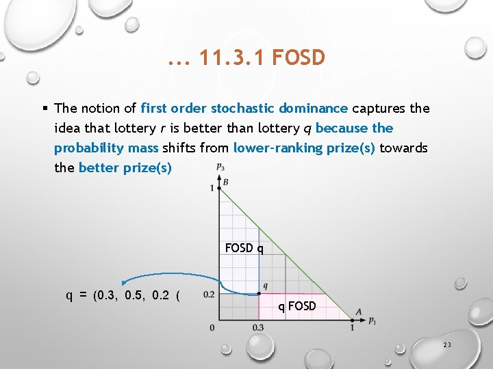
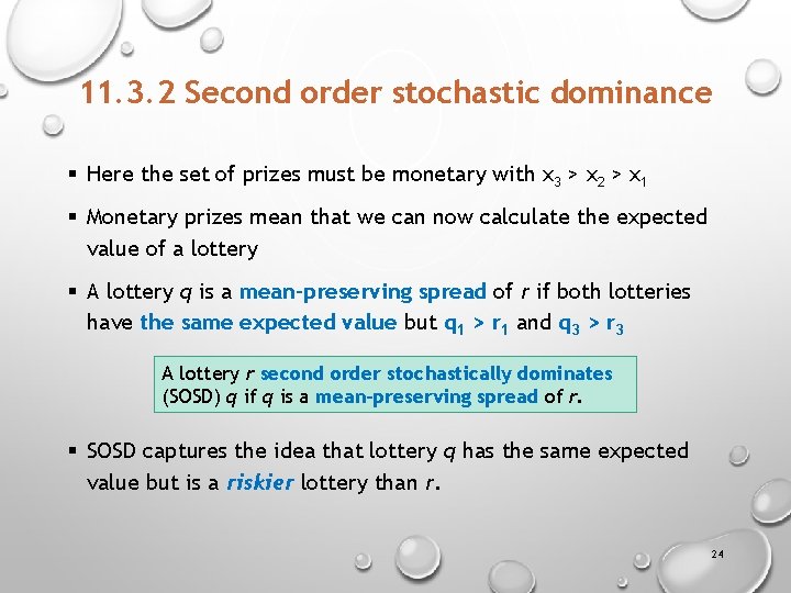
. . . 11. 3. 1 FOSD § The notion of first order stochastic dominance captures the idea that lottery r is better than lottery q because the probability mass shifts from lower-ranking prize(s) towards the better prize(s) FOSD q q = (0. 3, 0. 5, 0. 2 ( q FOSD 23

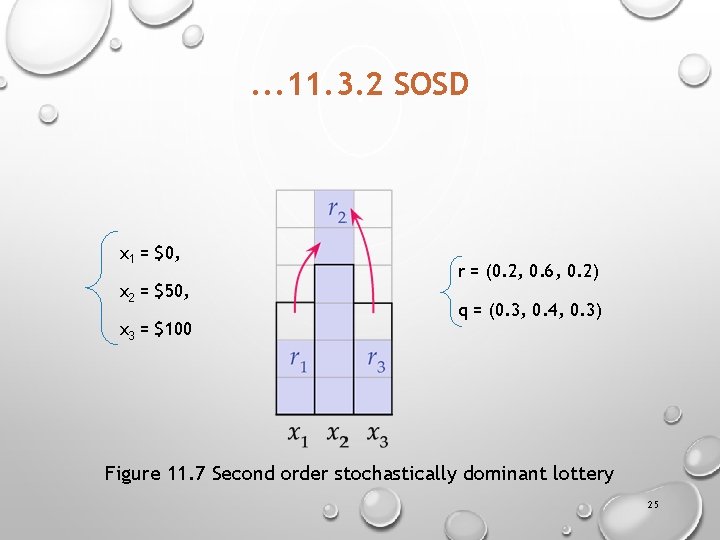
11. 3. 2 Second order stochastic dominance § Here the set of prizes must be monetary with x 3 > x 2 > x 1 § Monetary prizes mean that we can now calculate the expected value of a lottery § A lottery q is a mean-preserving spread of r if both lotteries have the same expected value but q 1 > r 1 and q 3 > r 3 A lottery r second order stochastically dominates (SOSD) q if q is a mean-preserving spread of r. § SOSD captures the idea that lottery q has the same expected value but is a riskier lottery than r. 24

. . . 11. 3. 2 SOSD x 1 = $0, x 2 = $50, x 3 = $100 r = (0. 2, 0. 6, 0. 2) q = (0. 3, 0. 4, 0. 3) Figure 11. 7 Second order stochastically dominant lottery 25

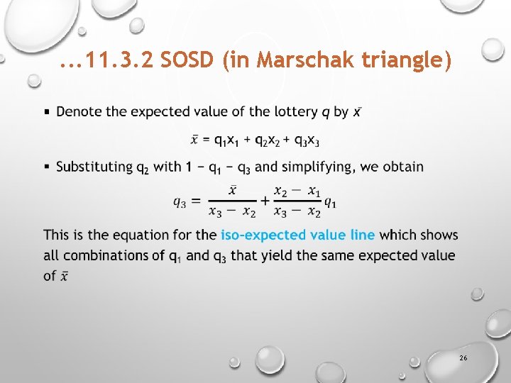
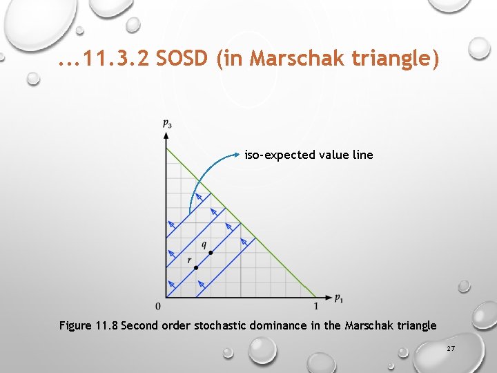
. . . 11. 3. 2 SOSD (in Marschak triangle) § 26

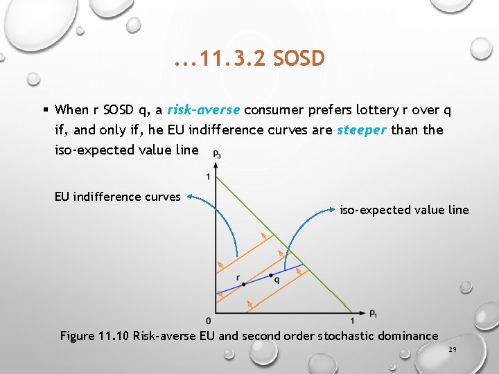
. . . 11. 3. 2 SOSD (in Marschak triangle) iso-expected value line Figure 11. 8 Second order stochastic dominance in the Marschak triangle 27

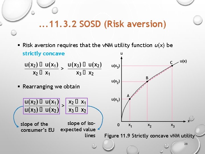
. . . 11. 3. 2 SOSD (Risk aversion) § Risk aversion requires that the v. NM utility function u(x) be strictly concave § Rearranging we obtain slope of the consumer’s EU slope of isoexpected value lines Figure 11. 9 Strictly concave v. NM utility 28

. . . 11. 3. 2 SOSD § When r SOSD q, a risk-averse consumer prefers lottery r over q if, and only if, he EU indifference curves are steeper than the iso-expected value line EU indifference curves iso-expected value line Figure 11. 10 Risk-averse EU and second order stochastic dominance 29

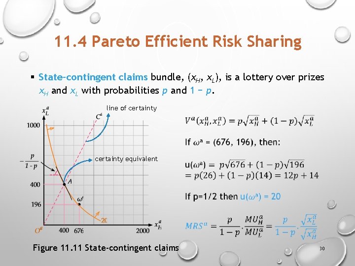
11. 4 Pareto Efficient Risk Sharing § State-contingent claims bundle, (x. H, x. L), is a lottery over prizes x. H and x. L with probabilities p and 1 − p. line of certainty equivalent Figure 11. 11 State-contingent claims 30

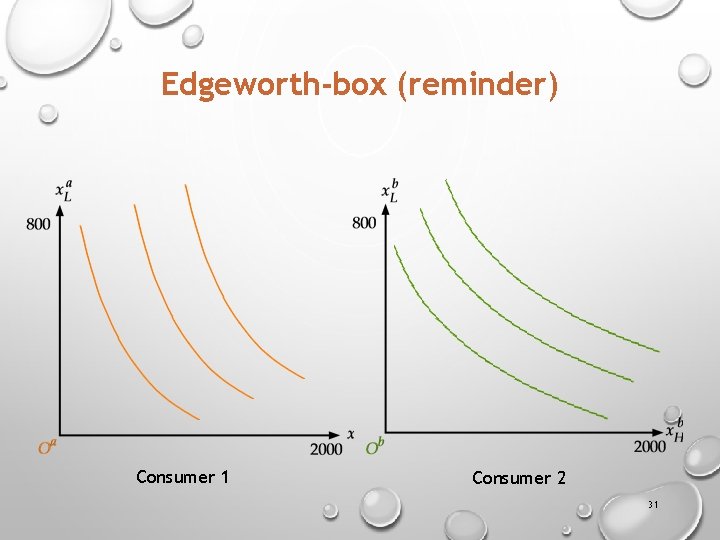
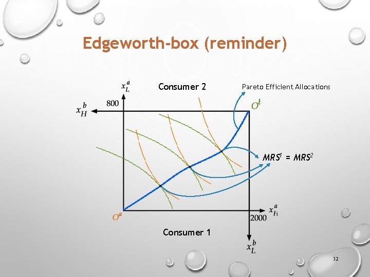
Edgeworth-box (reminder) Consumer 1 Consumer 2 31

Edgeworth-box (reminder) Consumer 2 Pareto Efficient Allocations MRS 1 = MRS 2 Consumer 1 32

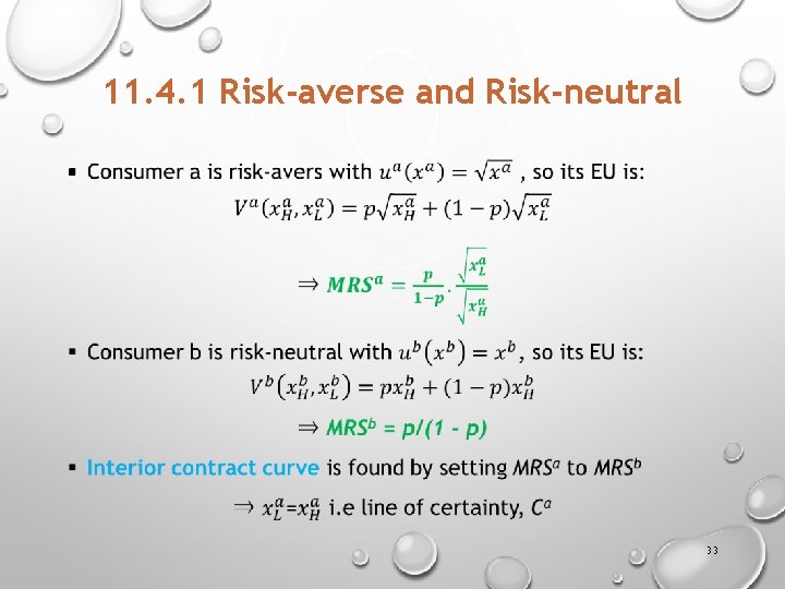
11. 4. 1 Risk-averse and Risk-neutral § 33

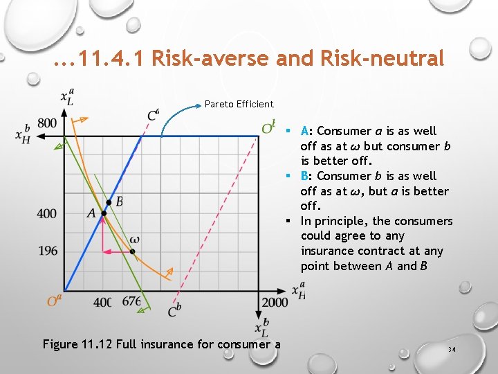
. . . 11. 4. 1 Risk-averse and Risk-neutral Pareto Efficient § A: Consumer a is as well off as at ω but consumer b is better off. § B: Consumer b is as well off as at ω, but a is better off. § In principle, the consumers could agree to any insurance contract at any point between A and B Figure 11. 12 Full insurance for consumer a 34

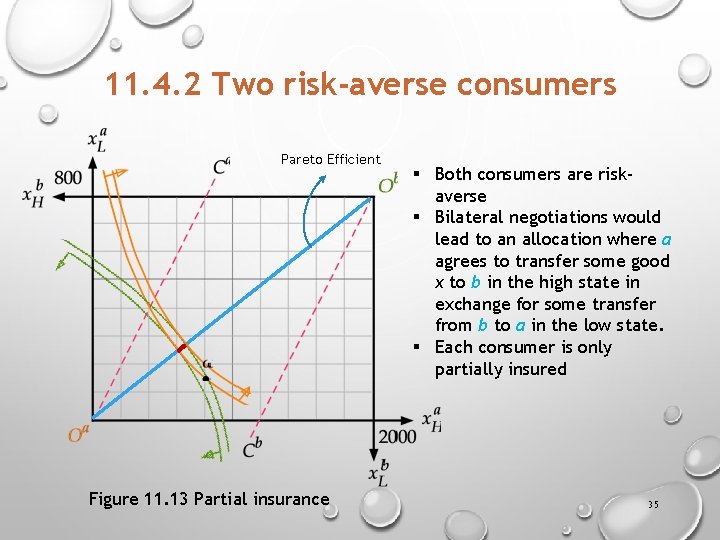
11. 4. 2 Two risk-averse consumers Pareto Efficient Figure 11. 13 Partial insurance § Both consumers are riskaverse § Bilateral negotiations would lead to an allocation where a agrees to transfer some good x to b in the high state in exchange for some transfer from b to a in the low state. § Each consumer is only partially insured 35