Explore the concepts of expectation standard deviation variance

Explore the concepts of expectation, standard deviation, variance, and covariance It is based on a lecture given by Professor Costis Maglaras at Columbia University.

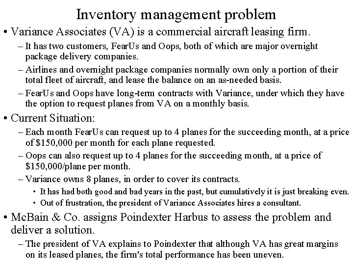
Inventory management problem • Variance Associates (VA) is a commercial aircraft leasing firm. – It has two customers, Fear. Us and Oops, both of which are major overnight package delivery companies. – Airlines and overnight package companies normally own only a portion of their total fleet of aircraft, and lease the balance on an as-needed basis. – Fear. Us and Oops have long-term contracts with Variance, under which they have the option to request planes from VA on a monthly basis. • Current Situation: – Each month Fear. Us can request up to 4 planes for the succeeding month, at a price of $150, 000 per month for each plane requested. – Oops can also request up to 4 planes for the succeeding month, at a price of $150, 000/plane per month. – Variance owns 8 planes, in order to cover its contracts. • It has had both good and bad years in the past, but cumulatively it is just breaking even. • Out of frustration, the president of Variance Associates hires a consultant. • Mc. Bain & Co. assigns Poindexter Harbus to assess the problem and deliver a solution. – The president of VA explains to Poindexter that although VA has great margins on its leased planes, the firm's total performance has been uneven.

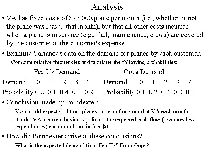
Analysis • VA has fixed costs of $75, 000/plane per month (i. e. , whether or not the plane was leased that month), but that all other costs incurred when a plane is in service (e. g. , fuel, maintenance, crews) are covered by the customer at the customer's expense. • Examine Variance's data on the demand for planes by each customer. Compute relative frequencies and tabulates the following probabilities: Fear. Us Demand Oops Demand 0 1 2 3 4 Demand 0 1 2 3 4 Probability 0. 2 0. 1 0. 4 0. 1 0. 2 Probability 0. 1 0. 2 0. 4 0. 2 0. 1 • Conclusion made by Poindexter: – VA should expect 4 of their planes to be on the ground at VA each month. – Under VA's current business policies, the expected cash flow (revenues less expenditures) each month are in fact $0. • How did Poindexter arrive at these conclusions? – What is the expected demand from Fear. Us? From Oops?

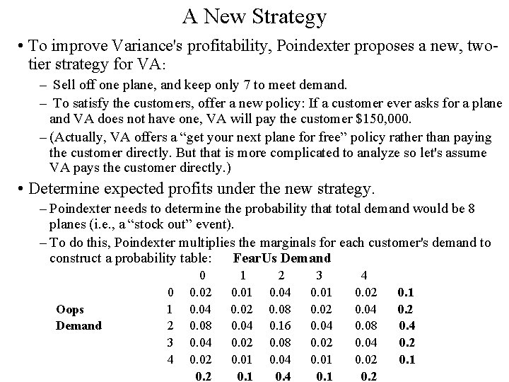
A New Strategy • To improve Variance's profitability, Poindexter proposes a new, twotier strategy for VA: – Sell off one plane, and keep only 7 to meet demand. – To satisfy the customers, offer a new policy: If a customer ever asks for a plane and VA does not have one, VA will pay the customer $150, 000. – (Actually, VA offers a “get your next plane for free” policy rather than paying the customer directly. But that is more complicated to analyze so let's assume VA pays the customer directly. ) • Determine expected profits under the new strategy. – Poindexter needs to determine the probability that total demand would be 8 planes (i. e. , a “stock out” event). – To do this, Poindexter multiplies the marginals for each customer's demand to construct a probability table: Fear. Us Demand 0 1 2 3 4 0 0. 02 0. 01 0. 04 0. 01 0. 02 0. 1 Oops 1 0. 04 0. 02 0. 08 0. 02 0. 04 0. 2 Demand 2 0. 08 0. 04 0. 16 0. 04 0. 08 0. 4 3 0. 04 0. 02 0. 08 0. 02 0. 04 0. 2 4 0. 02 0. 01 0. 04 0. 01 0. 02 0. 1 0. 2 0. 1 0. 4 0. 1 0. 2

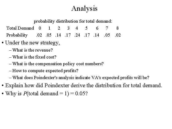
Analysis probability distribution for total demand: Total Demand 0 1 2 3 4 5 6 7 8 Probability . 02 . 05 . 14 . 17 . 24 . 17 . 14 . 05 . 02 • Under the new strategy, – What is the revenue? – What is the fixed cost? – What is the compensation policy cost numbers? – How to compute expected profits? – What does Poindexter's analysis indicate VA's expected profits will be? • Explain how did Poindexter derive the distribution for total demand. • Why is P(total demand = 1) = 0. 05?

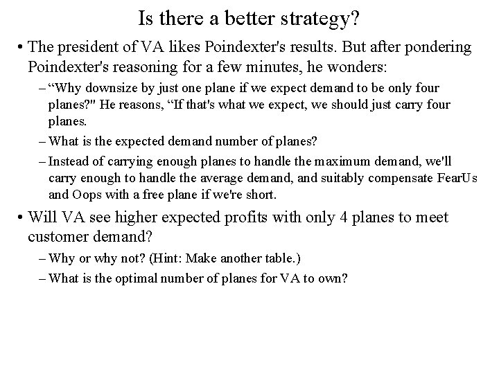
Is there a better strategy? • The president of VA likes Poindexter's results. But after pondering Poindexter's reasoning for a few minutes, he wonders: – “Why downsize by just one plane if we expect demand to be only four planes? " He reasons, “If that's what we expect, we should just carry four planes. – What is the expected demand number of planes? – Instead of carrying enough planes to handle the maximum demand, we'll carry enough to handle the average demand, and suitably compensate Fear. Us and Oops with a free plane if we're short. • Will VA see higher expected profits with only 4 planes to meet customer demand? – Why or why not? (Hint: Make another table. ) – What is the optimal number of planes for VA to own?

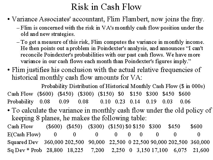
Risk in Cash Flow • Variance Associates' accountant, Flim Flambert, now joins the fray. – Flim is concerned with the risk in VA's monthly cash flow position under the old and new strategies. – To get a measure of this risk, Flim computes the variance in monthly income. He then points out a problem in Poindexter's analysis, and announces “I can't reconcile Poindexter's probabilities with our past cash flows. We have more variance in our cash flows each month than Poindexter's figures imply. ” • Flim justifies his conclusion with the actual relative frequencies of historical monthly cash flow amounts for VA: Probability Distribution of Historical Monthly Cash Flow ($ in 000 s) Cash Flow ($600) ($450) ($300) ($150) $0 $150 $300 $450 $600 Probability 0. 08 0. 09 0. 08 0. 10 0. 23 0. 14 0. 19 0. 03 0. 06 • To calculate the variance in monthly cash flow under the old policy of keeping 8 planes, he makes the following table: Cash Flow ($600) ($450) ($300) ($150) $0 $150 $300 $450 $600 E(Cash Flow) 0 0 0 0 0 0 Squared Dev 360, 000 202, 500 90, 000 22, 500 0 22, 500 90, 000 202, 500 360, 000 Sq Dev * Prob 28, 800 18, 225 7, 200 2, 250 0 3, 150 17, 100 6, 075 21, 600

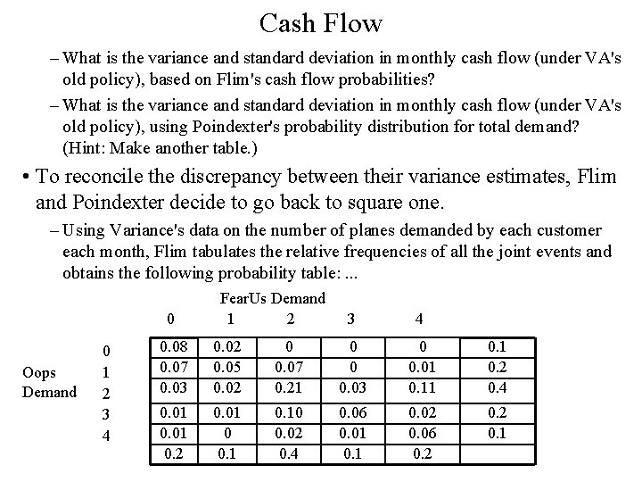
Cash Flow – What is the variance and standard deviation in monthly cash flow (under VA's old policy), based on Flim's cash flow probabilities? – What is the variance and standard deviation in monthly cash flow (under VA's old policy), using Poindexter's probability distribution for total demand? (Hint: Make another table. ) • To reconcile the discrepancy between their variance estimates, Flim and Poindexter decide to go back to square one. – Using Variance's data on the number of planes demanded by each customer each month, Flim tabulates the relative frequencies of all the joint events and obtains the following probability table: . . . Fear. Us Demand 0 1 2 3 4 0. 08 0 Oops Demand 1 2 3 4 0. 07 0. 03 0. 02 0. 05 0. 02 0 0. 07 0. 21 0 0 0. 03 0 0. 01 0. 2 0. 4 0. 01 0. 2 0. 01 0 0. 10 0. 02 0. 4 0. 06 0. 01 0. 02 0. 06 0. 2 0. 1

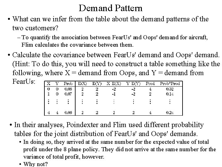
Demand Pattern • What can we infer from the table about the demand patterns of the two customers? – To quantify the association between Fear. Us' and Oops' demand for aircraft, Flim calculates the covariance between them. • Calculate the covariance between Fear. Us' demand Oops' demand. (Hint: To do this, you will need to construct a table something like the following, where X = demand from Oops, and Y = demand from Fear. Us: • In their analyses, Poindexter and Flim used different probability tables for the joint distribution of Fear. Us' and Oops' demands. • In doing so, they arrived at the same number for the expected value of total profit under the 8 plane policy. They did not arrive at the same number for the variance of total profit, however. • Why not?

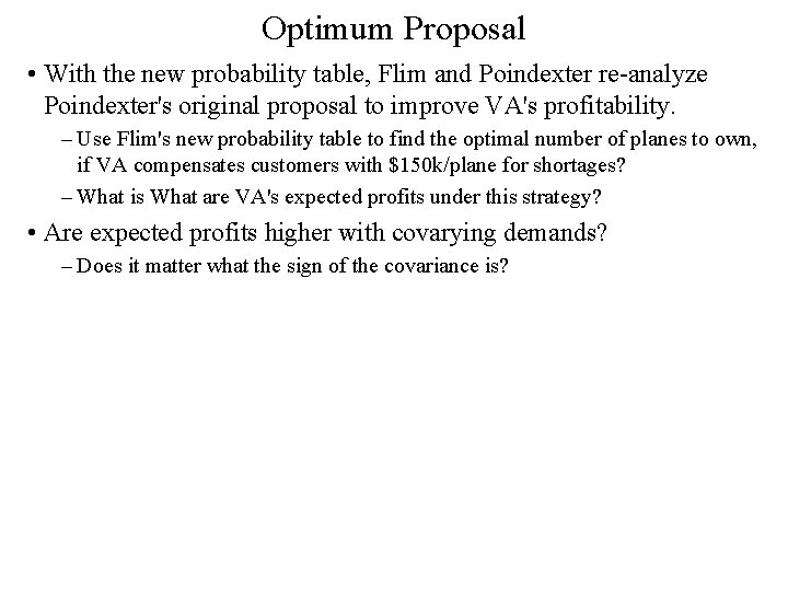
Optimum Proposal • With the new probability table, Flim and Poindexter re-analyze Poindexter's original proposal to improve VA's profitability. – Use Flim's new probability table to find the optimal number of planes to own, if VA compensates customers with $150 k/plane for shortages? – What is What are VA's expected profits under this strategy? • Are expected profits higher with covarying demands? – Does it matter what the sign of the covariance is?

Summary questions: • What is the optimal level of capacity for a firm facing uncertain demand: enough to cover maximum demand, average demand, or something else? – Why - what are we trading over here? – What information do we need to answer this for a particular firm? • If a firm has fixed costs and capacity constraints, which is better, to have customers whose demands positively covary or whose demands negatively covary? – What does this imply about the firm's capacity requirements and, given that, capital utilization rates?

Probability: the study of randomness

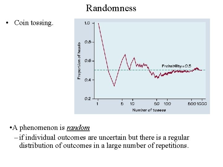
Randomness • Coin tossing. • A phenomenon is random – if individual outcomes are uncertain but there is a regular distribution of outcomes in a large number of repetitions.

Probability • The probability of any outcome of a random phenomenon is – long term relative frequency, i. e. • the proportion of the times the outcome would occur in a very long series of repetitions. (empirical) • Trials need to be independent. – Computer simulation is a good tool to study random behavior. • The uses of probability – Begins with gambling. – Now applied to analyze data in astronomy, mortality data, traffic flow, telephone interchange, genetics, epidemics, investment. . .

Probability Terms • Random Experiment: A process leading to at least 2 possible outcomes with uncertainty as to which will occur. • Event: An event is a subset of all possible outcomes of an experiment. – Intersection of Events: Let A and B be two events. Then the intersection of the two events, denoted A B, is the event that both A and B occur. – Union of Events: The union of the two events, denoted A B, is the event that A or B (or both) occurs. – Complement: Let A be an event. The complement of A (denoted ) is the event that A does not occur. – Mutually Exclusive Events: A and B are said to be mutually exclusive if at most one of the events A and B can occur. • Basic Outcomes: The simple indecomposable possible results of an experiment. One and exactly one of these outcomes must occur. The set of basic outcomes is mutually exclusive and collectively exhaustive. • Sample Space: The totality of basic outcomes of an experiment.

Basic Probability Rules 1. For any event A, 0 P(A) 1. 2. If A and B can never both occur (they are mutually exclusive), then P(A and B) = P(A B) = 0. 3. P(A or B) = P(A) + P(B) - P(A B). 4. If A and B are mutually exclusive events, then P(A or B) = P(A) + P(B). 5. P(Ac) = 1 - P(A). Independent Events • Two events A and B are said to be independent if the fact that A has occurred or not does not affect your assessment of the probability of B occurring. Conversely, the fact that B has occurred or not does not affect your assessment of the probability of A occurring. 6. If A and B are independent events, then P(A and B) = P(A) P(B). (Markov? ? )

Probability models • Two parts in coin tossing. – A list of possible outcomes. – A probability for each outcome. • The Sample space S of a random phenomenon is the set of all possible outcomes. – Examples. S={heads, tails}={H, T} – General analysis is possible.

• What is the probability of “exactly 2 heads in four tosses of a coin”? • What kind of rules that any assignment of probabilities must satisfy? • An event is an outcome or a set of outcomes. (= it is a subset of the sample space) • A={HHTT, HTHT, HTTH, THHT, THTH, TTHH} • In a probability model, events have probabilities that satisfy. . . • Two events A and B are independent if knowing that one occurs does not change the probability that the other occurs. • If A and B are independent, P(A and B) = P(A)P(B) the multiplication rule for independent events.

Independent/Dependent • The heads of successive coin tosses are {independent, not independent}. • The colors of successive cards dealt from the same deck are {independent, not independent}. • Two successive blood pressure measurements are {independent, not independent}. • Two successive IQ test results are {independent, not independent}

Conditional Probability • Example: One of the businesses that have grown out of the public's increased use of the internet has been providing internet service to individual customers; those who provide this service are called Internet Service Providers (ISPs). – More recently, a number of ISPs have developed business models whereby they do not need to charge customers for internet service at all, by collecting fees from advertisers, and forcing the non-paying customers to view these advertisements. – Jupiter Communications estimates that by the end of 2003 20% of web users will have a free ISP. 6% of all web users, it is estimated, will have both a free ISP and a paid ISP account. • In 2003, what proportion of internet users is expected to do the following? a) subscribes to both a free ISP and a paid ISP. b) subscribes only to a paid ISP. c) subscribes only to a free ISP.

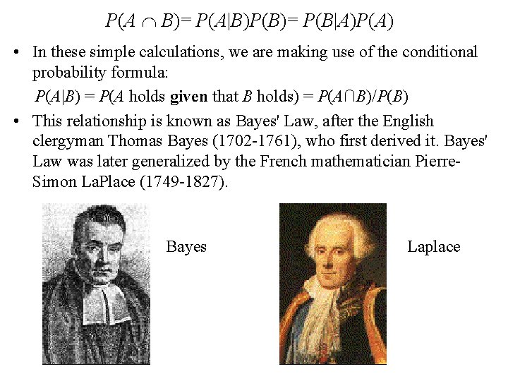
P(A B)= P(A|B)P(B)= P(B|A)P(A) • In these simple calculations, we are making use of the conditional probability formula: P(A|B) = P(A holds given that B holds) = P(A∩B)/P(B) • This relationship is known as Bayes' Law, after the English clergyman Thomas Bayes (1702 -1761), who first derived it. Bayes' Law was later generalized by the French mathematician Pierre. Simon La. Place (1749 -1827). Bayes Laplace

Random Variables • A random variable is a variable whose value is a numerical outcome of a random phenomenon. – Sample spaces need not consist of numbers. – Examples: number of heads in 4 coin tossing, …

Random Variable • A random variable is called discrete if it has countably many possible values; otherwise, it is called continuous. • The following quantities would typically be modeled as discrete random variables: – The number of defects in a batch of 20 items. – The number of people preferring one brand over another in a market research study. – The credit rating of a debt issue at some date in the future. • The following would typically be modeled as continuous random variables: – The yield on a 10 -year Treasury bond three years from today. – The proportion of defects in a batch of 10, 000 items. – The time between breakdowns of a machine. –Sometimes, we approximate a discrete random variable with a continuous one if the possible values are very close together; e. g. , stock prices are often treated as continuous random variables.

Distribution: discrete • If X is a discrete random variable then we denote its pmf by PX. – The rule that assigns specific probabilities to specific values for a discrete random variable is called its probability mass function or pmf. – For any value x, PX(x) is the probability of the event that X = x; i. e. , PX(x) = P(X = x) = probability that the value of X is x. – We always use capital letters for random variables. Lower-case letters like x and y stand for possible values (i. e. , numbers) and are not random. – A pmf is graphed by drawing a vertical line of height PX(x) at each possible value x. • It is similar to a histogram, except that the height of the line (or bar) gives theoretical probability rather than the observed frequency. • Are a histogram close to its corresponding pmf? • The pmf gives us one way to describe the distribution of a random variable. Another way is provided by the cumulative probability function, denoted by FX and defined by FX(x) = P(X≦ x) – It is the probability that X is less than or equal to x. – The the pmf gives the probability that the random variable lands on a particular value, the cpf gives the probability that it lands on or below a particular value. In particular, FX is always an increasing function.

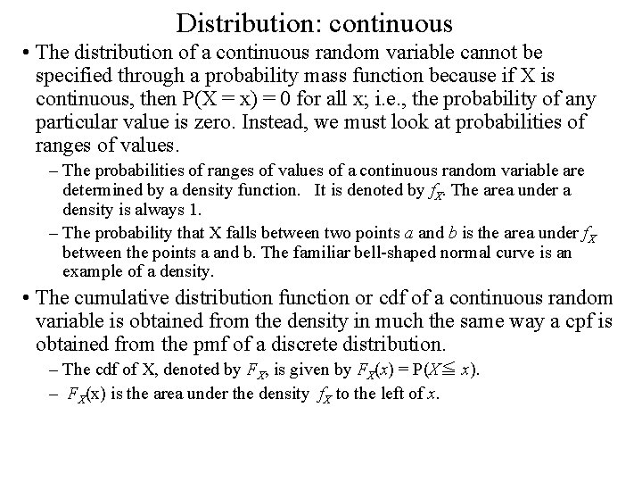
Distribution: continuous • The distribution of a continuous random variable cannot be specified through a probability mass function because if X is continuous, then P(X = x) = 0 for all x; i. e. , the probability of any particular value is zero. Instead, we must look at probabilities of ranges of values. – The probabilities of ranges of values of a continuous random variable are determined by a density function. It is denoted by f. X. The area under a density is always 1. – The probability that X falls between two points a and b is the area under f. X between the points a and b. The familiar bell-shaped normal curve is an example of a density. • The cumulative distribution function or cdf of a continuous random variable is obtained from the density in much the same way a cpf is obtained from the pmf of a discrete distribution. – The cdf of X, denoted by FX, is given by FX(x) = P(X≦ x). – FX(x) is the area under the density f. X to the left of x.

Expectation • The expected value of a random variable is denoted by E[X]. –It can be thought of as the “average” value attained by the random variable. –The expected value of a random variable is also called its mean, in which case we use the notation X. –The formula for the expected value of a discrete random variable is this: E[X] =Sx x. PX(x). –The expected value is the sum, over all possible values x, of x times its probability PX(x). –The expected value of a continuous random variable cannot be expressed as a sum; instead it is an integral involving the density. • If g is a function (for example, g(x) = x 2), then the expected value of g(X) is E[g(X)] =Sx x 2 PX(x). • The variance of a random variable X is denoted by either Var[X] or X 2. –The variance is defined by X 2 = E[(X- X)2]= E[X 2] - (E[X])2. –For a discrete distribution, we can write the variance as Sx (x- X)2 PX(x).

Discrete random variable • Discrete random variable X has a finite number of possible values. • The probability distribution of X lists the values and their probabilities. – The probabilities pk must satisfy. . . • Every probability pi is a number between 0 and 1. • p 1+ p 2+. . . +pk=1. • The probability of any event is found by adding the probabilities pi of the particular values xi that make up the event.

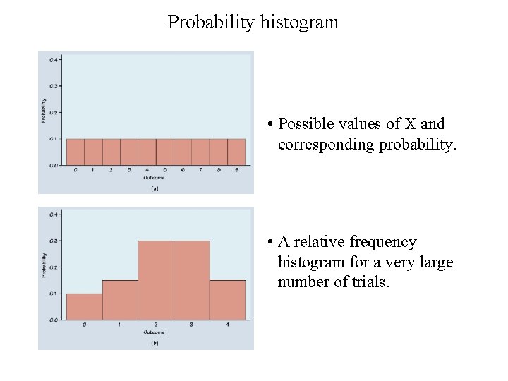
Probability histogram • Possible values of X and corresponding probability. • A relative frequency histogram for a very large number of trials.

Commonly Used Continuous Distribution The Normal Distribution • History: –Abraham de Moivre (1667 -1754) first described the normal distribution in 1733. –Adolphe Quetelet (1796 -1874) used the normal distribution to describe the concept of l'homme moyen (the average man), thus popularizing the notion of the bell-shaped curve. –Carl Friedrich Gauss (1777 -1855) used the normal distribution to describe measurement errors in geography and astronomy.

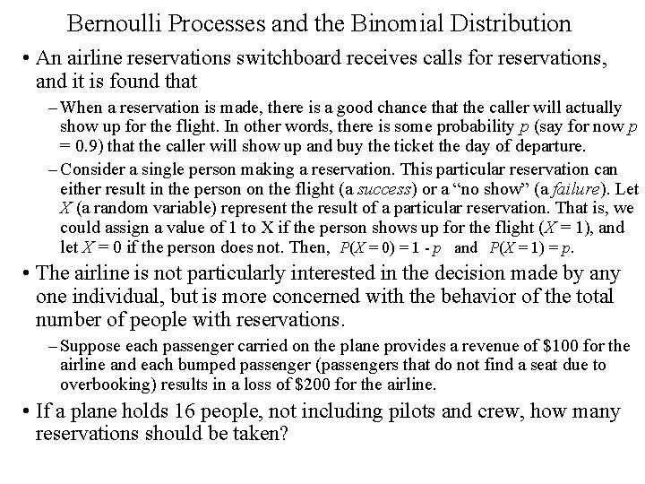
Bernoulli Processes and the Binomial Distribution • An airline reservations switchboard receives calls for reservations, and it is found that – When a reservation is made, there is a good chance that the caller will actually show up for the flight. In other words, there is some probability p (say for now p = 0. 9) that the caller will show up and buy the ticket the day of departure. – Consider a single person making a reservation. This particular reservation can either result in the person on the flight (a success) or a “no show” (a failure). Let X (a random variable) represent the result of a particular reservation. That is, we could assign a value of 1 to X if the person shows up for the flight (X = 1), and let X = 0 if the person does not. Then, P(X = 0) = 1 - p and P(X = 1) = p. • The airline is not particularly interested in the decision made by any one individual, but is more concerned with the behavior of the total number of people with reservations. – Suppose each passenger carried on the plane provides a revenue of $100 for the airline and each bumped passenger (passengers that do not find a seat due to overbooking) results in a loss of $200 for the airline. • If a plane holds 16 people, not including pilots and crew, how many reservations should be taken?

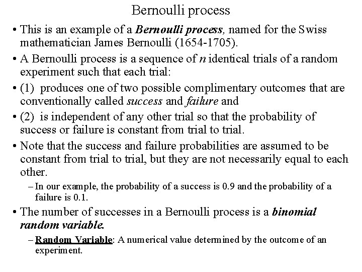
Bernoulli process • This is an example of a Bernoulli process, named for the Swiss mathematician James Bernoulli (1654 -1705). • A Bernoulli process is a sequence of n identical trials of a random experiment such that each trial: • (1) produces one of two possible complimentary outcomes that are conventionally called success and failure and • (2) is independent of any other trial so that the probability of success or failure is constant from trial to trial. • Note that the success and failure probabilities are assumed to be constant from trial to trial, but they are not necessarily equal to each other. – In our example, the probability of a success is 0. 9 and the probability of a failure is 0. 1. • The number of successes in a Bernoulli process is a binomial random variable. – Random Variable: A numerical value determined by the outcome of an experiment.

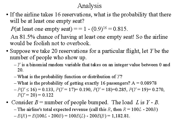
Analysis • If the airline takes 16 reservations, what is the probability that there will be at least one empty seat? P(at least one empty seat) = = 1 - (0. 9)16 = 0. 815. An 81. 5% chance of having at least one empty seat! So the airline would be foolish not to overbook. • Suppose we take 20 reservations for a particular flight, let Y be the number of people who show up. – Y is a binomial random variable that takes on an integer value between 0 and 20. – What is the probability function or distribution of Y? – What is the probability of getting exactly 16 passengers? A = 0. 08978 – P(Y 16) = 0. 133, P(Y = 17)= 0. 190, P(Y = 18)=0. 285, P(Y = 19)= 0. 270, P(Y = 20) = 0. 122 • Consider B = number of people bumped. The load L is Y - B. – The airline's total expected revenue (call this R, then R = 100 L - 200 B) – E(R) = E(100 L - 200 B) = 100 E(L) - 200 E(B) = 1, 182. 81.

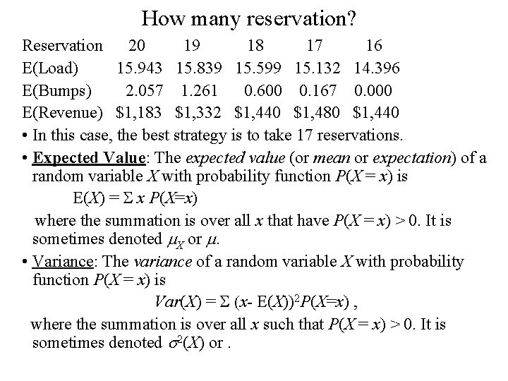
How many reservation? Reservation 20 19 18 17 16 E(Load) 15. 943 15. 839 15. 599 15. 132 14. 396 E(Bumps) 2. 057 1. 261 0. 600 0. 167 0. 000 E(Revenue) $1, 183 $1, 332 $1, 440 $1, 480 $1, 440 • In this case, the best strategy is to take 17 reservations. • Expected Value: The expected value (or mean or expectation) of a random variable X with probability function P(X = x) is E(X) = S x P(X=x) where the summation is over all x that have P(X = x) > 0. It is sometimes denoted X or . • Variance: The variance of a random variable X with probability function P(X = x) is Var(X) = S (x- E(X))2 P(X=x) , where the summation is over all x such that P(X = x) > 0. It is sometimes denoted 2(X) or.