CEE 795 Water Resources Modeling and GIS Lecture

CEE 795 Water Resources Modeling and GIS Lecture 8: Hydrologic Modeling and AGWA April 3, 2006 Learning Objectives: • Describe the steps in hydrologic modeling • Evaluate different types of hydrologic models • Summarize the components of AGWA Handouts: Assignments:

Hydrologic/Watershed Modeling Thomas Piechota, Ph. D. , P. E. Department of Civil and Environmental Engineering University of Nevada, Las Vegas piechota@ce. unlv. edu

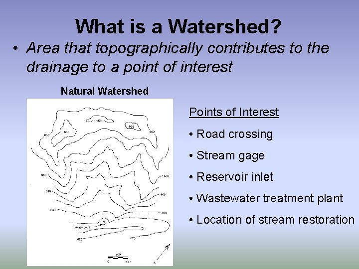
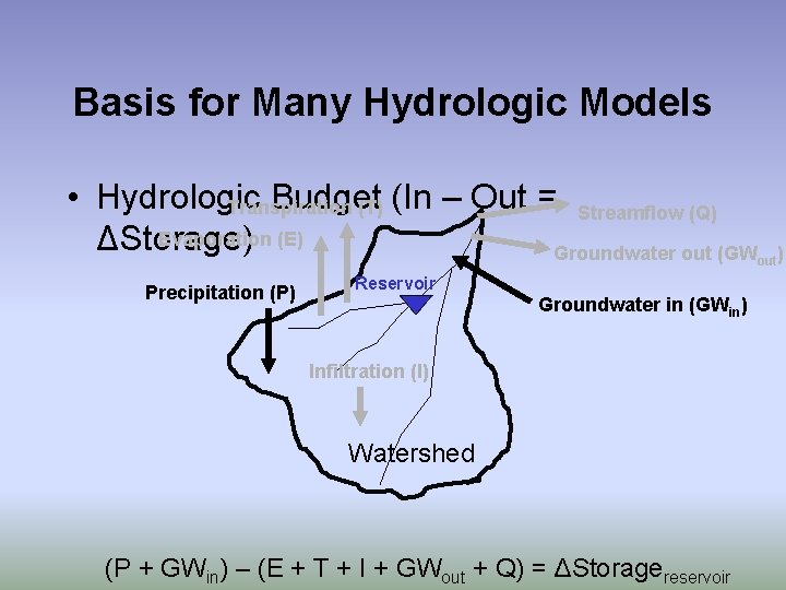
Definitions • Watershed: area that topographically contributes to the drainage to a point of interest • Streamflow: runoff (rate or volume) at a specified point in a watershed. • Hydrologic budget: accounting of water in a system.

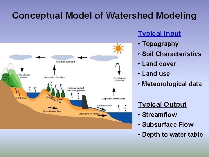
Conceptual Model of Watershed Modeling Typical Input • Topography • Soil Characteristics • Land cover • Land use • Meteorological data Typical Output • Streamflow • Subsurface Flow • Depth to water table

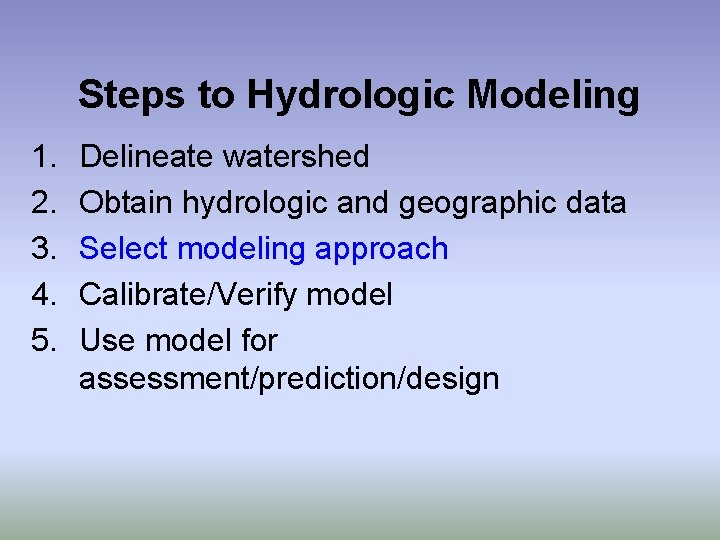
Steps to Hydrologic Modeling 1. 2. 3. 4. 5. Delineate watershed Obtain hydrologic and geographic data Select modeling approach Calibrate/Verify model Use model for assessment/prediction/design

What is a Watershed? • Area that topographically contributes to the drainage to a point of interest Natural Watershed Points of Interest • Road crossing • Stream gage • Reservoir inlet • Wastewater treatment plant • Location of stream restoration

Urban Watershed

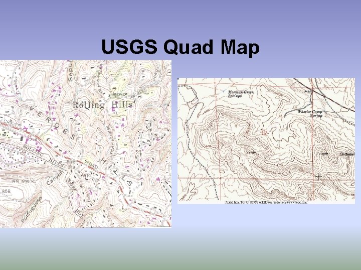
USGS Quad Map

Digital Elevation Model (DEM) • Digital file that stores the elevation of the land surface a specified grid cell size (e. g. , 30 meters)

Steps to Hydrologic Modeling 1. 2. 3. 4. 5. Delineate watershed Obtain hydrologic and geographic data Select modeling approach Calibrate/Verify model Use model for assessment/prediction/design

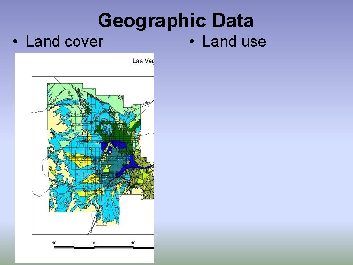
Geographic Data • Land cover • Land use

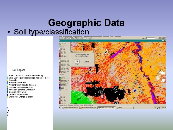
Geographic Data • Soil type/classification

Hydrologic Data • Meteorological Data – – Temperature Precipitation Wind speed Humidity • Extrapolation of point measurements – Theissen Polygons – Inverse distance weighting

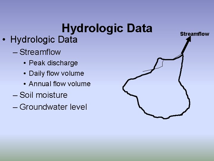
Hydrologic Data • Hydrologic Data – Streamflow • Peak discharge • Daily flow volume • Annual flow volume – Soil moisture – Groundwater level Streamflow

Steps to Hydrologic Modeling 1. 2. 3. 4. 5. Delineate watershed Obtain hydrologic and geographic data Select modeling approach Calibrate/Verify model Use model for assessment/prediction/design

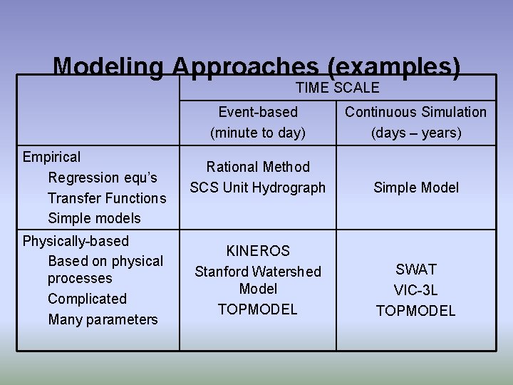
Modeling Approaches (examples) TIME SCALE Empirical Regression equ’s Transfer Functions Simple models Physically-based Based on physical processes Complicated Many parameters Event-based (minute to day) Continuous Simulation (days – years) Rational Method SCS Unit Hydrograph Simple Model KINEROS Stanford Watershed Model TOPMODEL SWAT VIC-3 L TOPMODEL

Basis for Many Hydrologic Models • Hydrologic Budget Transpiration (T) (In – Out = Streamflow (Q) Evaporation (E) ΔStorage) Groundwater out (GW Precipitation (P) Reservoir Groundwater in (GWin) Infiltration (I) Watershed (P + GWin) – (E + T + I + GWout + Q) = ΔStoragereservoir out)

Which Model Should be Used? • It Depends on: – What time scale are you working at? – What hydrologic quantity are you trying to obtain? – What data do you have for your watershed? – How fast of a computer do you have?

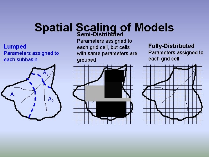
Spatial Scaling of Models Semi-Distributed Lumped Parameters assigned to each subbasin A 3 A 1 A 2 Parameters assigned to each grid cell, but cells with same parameters are grouped Fully-Distributed Parameters assigned to each grid cell

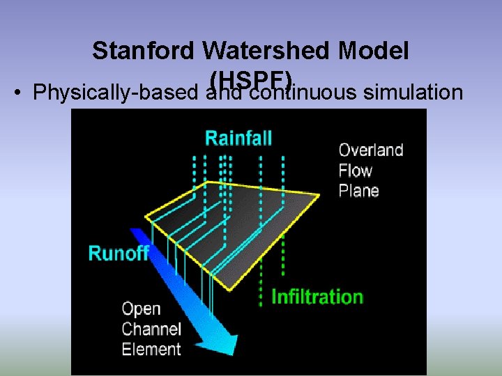
Stanford Watershed Model (HSPF) • Physically-based and continuous simulation

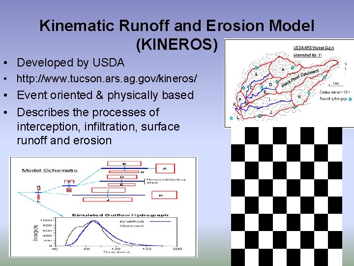
Kinematic Runoff and Erosion Model (KINEROS) • Developed by USDA • http: //www. tucson. ars. ag. gov/kineros/ • Event oriented & physically based • Describes the processes of interception, infiltration, surface runoff and erosion

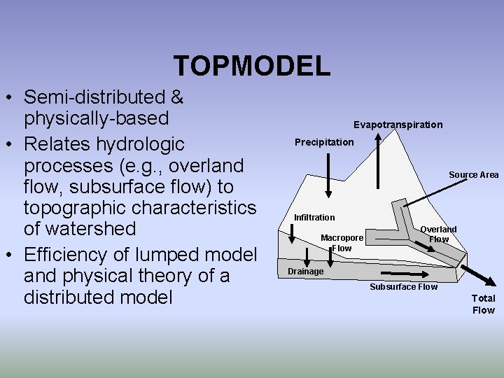
TOPMODEL • Semi-distributed & physically-based • Relates hydrologic processes (e. g. , overland flow, subsurface flow) to topographic characteristics of watershed • Efficiency of lumped model and physical theory of a distributed model Evapotranspiration Precipitation Source Area Infiltration Macropore Flow Overland Flow Drainage Subsurface Flow Total Flow

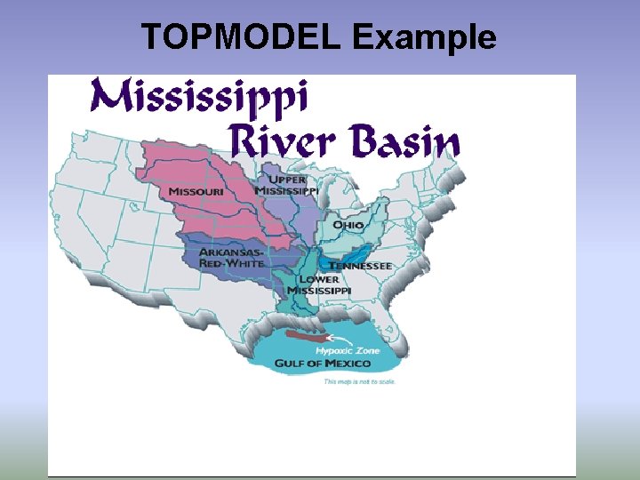
TOPMODEL Example

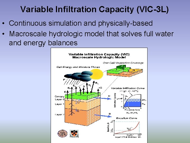
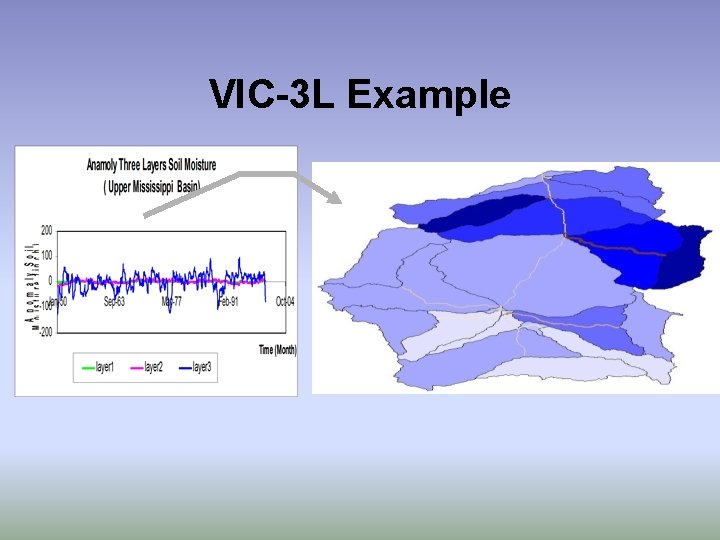
Variable Infiltration Capacity (VIC-3 L) • Continuous simulation and physically-based • Macroscale hydrologic model that solves full water and energy balances

VIC-3 L Example

Steps to Hydrologic Modeling 1. 2. 3. 4. 5. Delineate watershed Obtain hydrologic and geographic data Select modeling approach Calibrate/Verify model Use model for assessment/prediction/design

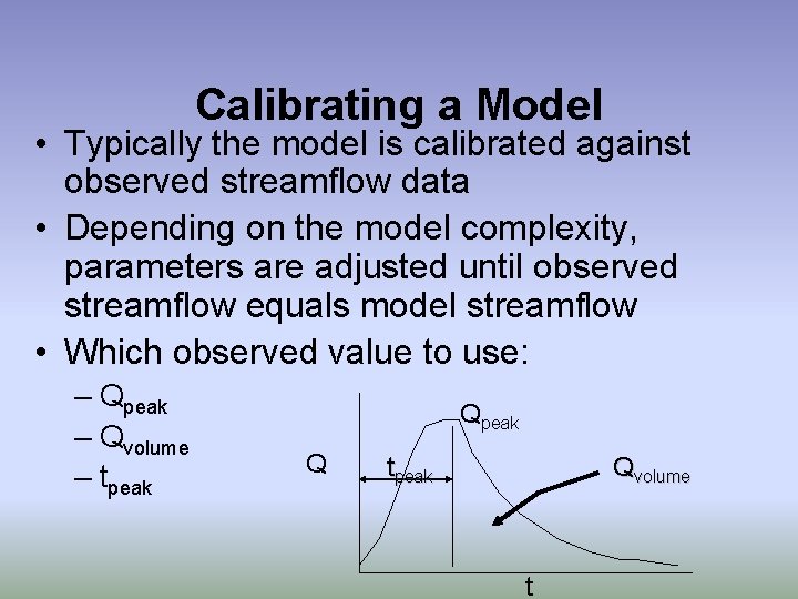
Calibrating a Model • Typically the model is calibrated against observed streamflow data • Depending on the model complexity, parameters are adjusted until observed streamflow equals model streamflow • Which observed value to use: – Qpeak – Qvolume – tpeak Qvolume t

Sensitive Parameters • Precipitation • Soil parameters – Hydraulic conductivity – Soil water holding capacity • Evaporation (for continuous simulation) • Flow routing parameters (for eventbased)

Uncertainties • Precipitation – Extrapolation of point to other areas – Temporal resolution of data • Soils information – Surveys are based on site visits and then extrapolated • Routing parameters – Usually assigned based on empirical studies

Steps to Hydrologic Modeling 1. 2. 3. 4. 5. Delineate watershed Obtain hydrologic and geographic data Select modeling approach Calibrate/Verify model Use model for assessment/prediction/design

Use of Models • Assessment – What happens if land use/land cover is changed? • Prediction – Flood forecasting • Design – How much flow will occur in a 100 year storm?

AUTOMATED GEOSPATIAL WATERSHED ASSESSMENT A GIS-BASED WATERSHED MODELING TOOL William Kepner and Darius Semmens US – EPA Landscape Ecology Branch Las Vegas, NV David Goodrich, Mariano Hernandez, Shea Burns, Averill Cate, Soren Scott, and Lainie Levick USDA-ARS Southwest Watershed Research Center, Tucson, AZ Phillip Guertin University of Arizona, Tucson, AZ Scott Miller University of Wyoming, Laramie, WY

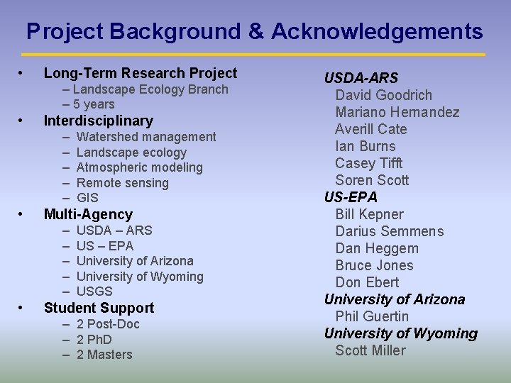
Project Background & Acknowledgements • Long-Term Research Project – Landscape Ecology Branch – 5 years • Interdisciplinary – – – • Multi-Agency – – – • Watershed management Landscape ecology Atmospheric modeling Remote sensing GIS USDA – ARS US – EPA University of Arizona University of Wyoming USGS Student Support – 2 Post-Doc – 2 Ph. D – 2 Masters USDA-ARS David Goodrich Mariano Hernandez Averill Cate Ian Burns Casey Tifft Soren Scott US-EPA Bill Kepner Darius Semmens Dan Heggem Bruce Jones Don Ebert University of Arizona Phil Guertin University of Wyoming Scott Miller

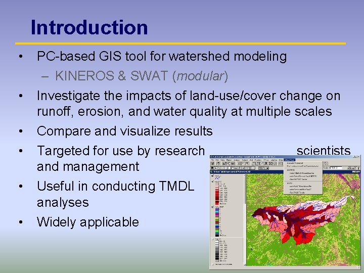
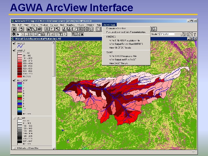
Introduction • • • PC-based GIS tool for watershed modeling – KINEROS & SWAT (modular) Investigate the impacts of land-use/cover change on runoff, erosion, and water quality at multiple scales Compare and visualize results Targeted for use by research scientists and management specialists Useful in conducting TMDL analyses Widely applicable

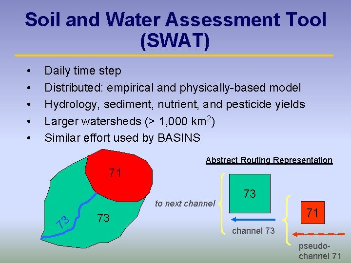
Soil and Water Assessment Tool (SWAT) • • • Daily time step Distributed: empirical and physically-based model Hydrology, sediment, nutrient, and pesticide yields Larger watersheds (> 1, 000 km 2) Similar effort used by BASINS Abstract Routing Representation 71 to next channel 73 73 71 73 channel 73 pseudochannel 71

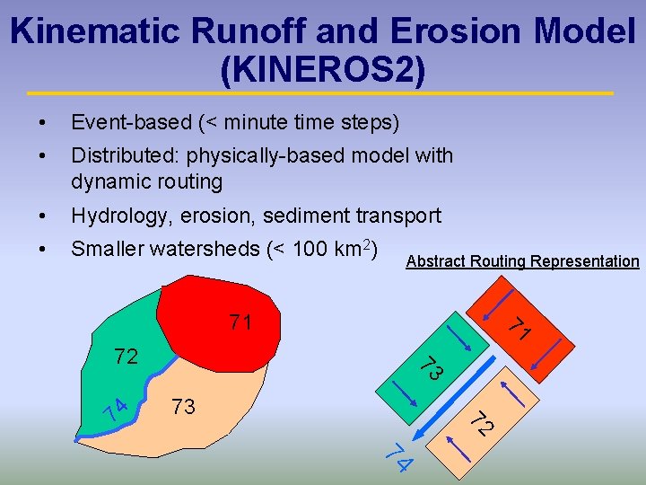
Kinematic Runoff and Erosion Model (KINEROS 2) • Event-based (< minute time steps) • Distributed: physically-based model with dynamic routing • Hydrology, erosion, sediment transport • Smaller watersheds (< 100 km 2) Abstract Routing Representation 71 71 73 72 74

AGWA Arc. View Interface

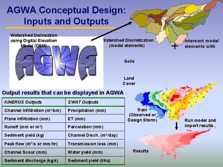
AGWA Conceptual Design: Inputs and Outputs Watershed Delineation using Digital Elevation Model (DEM) Watershed Discretization (model elements) + Intersect model elements with Soils Land Cover Output results that can be displayed in AGWA KINEROS Outputs SWAT Outputs Channel Infiltration (m 3/km) Precipitation (mm) Plane Infiltration (mm) ET (mm) Runoff (mm or m 3) Percolation (mm) Sediment yield (kg) Channel Disch. (m 3/day) Peak flow (m 3/s or mm/hr) Transmission loss (mm) Channel Scour (mm) Water yield (mm) Sediment discharge (kg/s) Sediment yield (t/ha) Rain (Observed or Design Storm) Results Run model and import results

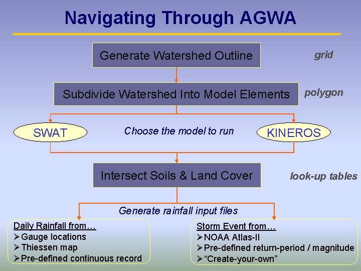
Navigating Through AGWA Generate Watershed Outline grid Subdivide Watershed Into Model Elements polygon SWAT Choose the model to run Intersect Soils & Land Cover KINEROS look-up tables Generate rainfall input files Daily Rainfall from… ØGauge locations ØThiessen map ØPre-defined continuous record Storm Event from… ØNOAA Atlas-II ØPre-defined return-period / magnitude Ø“Create-your-own”

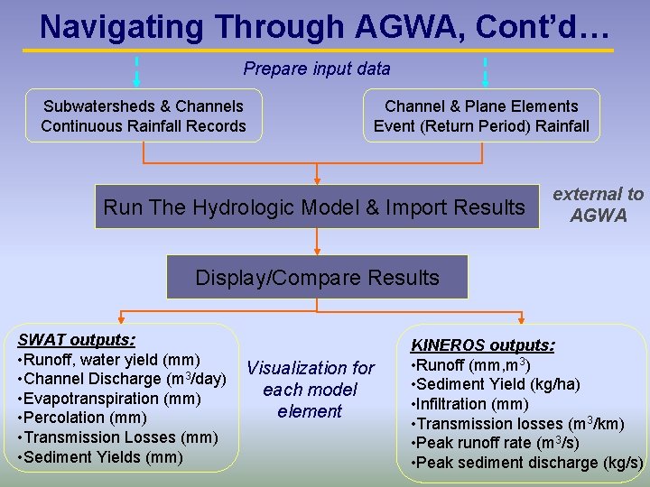
Navigating Through AGWA, Cont’d… Prepare input data Subwatersheds & Channels Continuous Rainfall Records Channel & Plane Elements Event (Return Period) Rainfall Run The Hydrologic Model & Import Results external to AGWA Display/Compare Results SWAT outputs: • Runoff, water yield (mm) • Channel Discharge (m 3/day) • Evapotranspiration (mm) • Percolation (mm) • Transmission Losses (mm) • Sediment Yields (mm) Visualization for each model element KINEROS outputs: • Runoff (mm, m 3) • Sediment Yield (kg/ha) • Infiltration (mm) • Transmission losses (m 3/km) • Peak runoff rate (m 3/s) • Peak sediment discharge (kg/s)

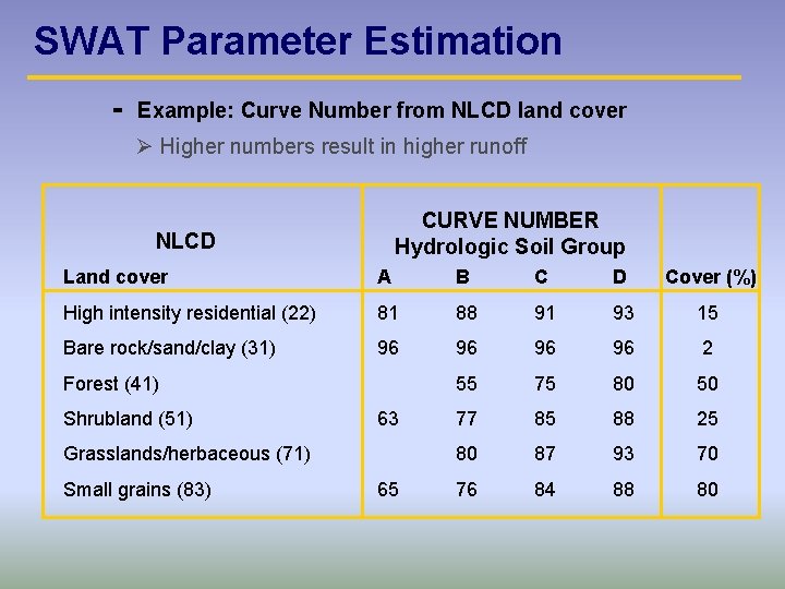
SWAT Parameter Estimation - Example: Curve Number from NLCD land cover Ø Higher numbers result in higher runoff CURVE NUMBER Hydrologic Soil Group NLCD Land cover A B C D Cover (%) High intensity residential (22) 81 88 91 93 15 Bare rock/sand/clay (31) 96 96 2 55 75 80 50 77 85 88 25 80 87 93 70 76 84 88 80 Forest (41) Shrubland (51) 63 Grasslands/herbaceous (71) Small grains (83) 65

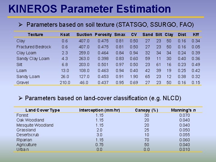
KINEROS Parameter Estimation Ø Parameters based on soil texture (STATSGO, SSURGO, FAO) Texture Clay Fractured Bedrock Clay Loam Sandy Clay Loam Silt Loam Sandy Loam Gravel Ksat 0. 6 2. 3 4. 3 6. 8 13. 0 26. 0 210. 0 Suction Porosity Smax 407. 0 0. 475 0. 81 259. 0 0. 464 0. 84 263. 0 0. 398 0. 83 203. 0 0. 501 0. 97 108. 0 0. 463 0. 94 127. 0 0. 453 0. 91 46. 0 0. 437 0. 95 CV 0. 50 0. 94 0. 60 0. 50 0. 40 1. 90 0. 69 Sand 27 27 32 59 23 42 65 27 Silt Clay 23 50 34 34 11 30 61 16 39 19 23 12 23 50 Dist 0. 16 0. 24 0. 40 0. 23 0. 25 0. 38 0. 16 Kff 0. 34 0. 05 0. 39 0. 36 0. 49 0. 42 0. 32 0. 15 Ø Parameters based on land-cover classification (e. g. NLCD) Land Cover Type Forest Oak Woodland Mesquite Woodland Grassland Desertscrub Riparian Agriculture Urba n Interception (mm/hr) 1. 15 2. 0 3. 0 1. 15 0. 75 0. 0 Canopy (%) 30 20 20 25 10 70 50 0. 0 Manning's n 0. 070 0. 040 0. 055 0. 060 0. 040 0. 010

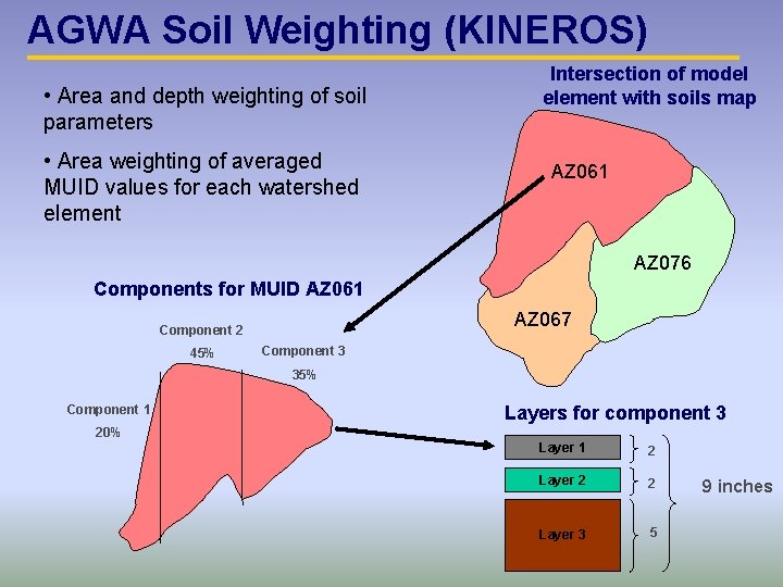
AGWA Soil Weighting (KINEROS) • Area and depth weighting of soil parameters • Area weighting of averaged MUID values for each watershed element Intersection of model element with soils map AZ 061 AZ 076 Components for MUID AZ 061 AZ 067 Component 2 45% Component 3 35% Component 1 Layers for component 3 20% Layer 1 2 Layer 2 2 Layer 3 5 9 inches

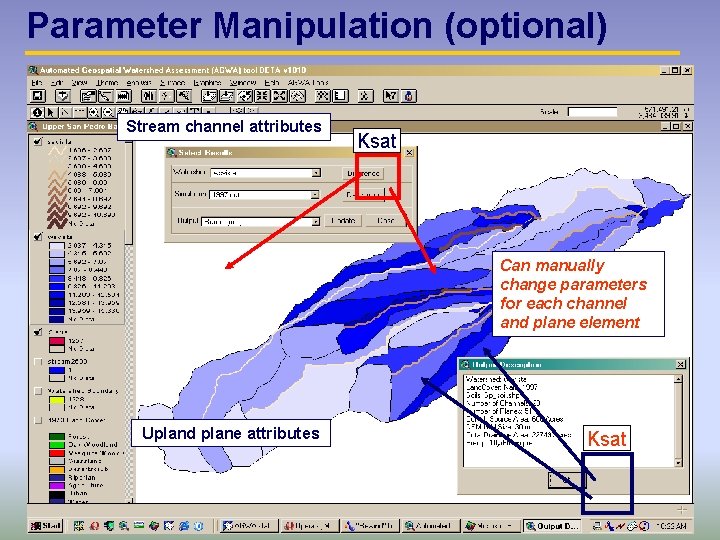
Parameter Manipulation (optional) Stream channel attributes Ksat Can manually change parameters for each channel and plane element Upland plane attributes Ksat

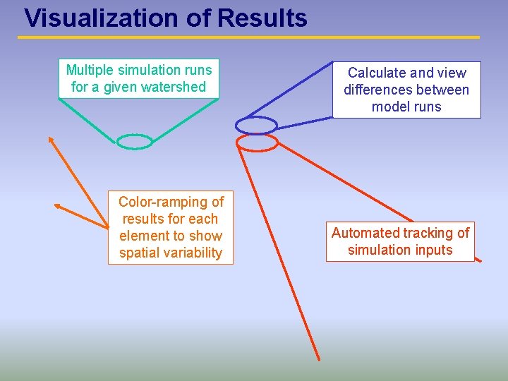
Visualization of Results Multiple simulation runs for a given watershed Color-ramping of results for each element to show spatial variability Calculate and view differences between model runs Automated tracking of simulation inputs

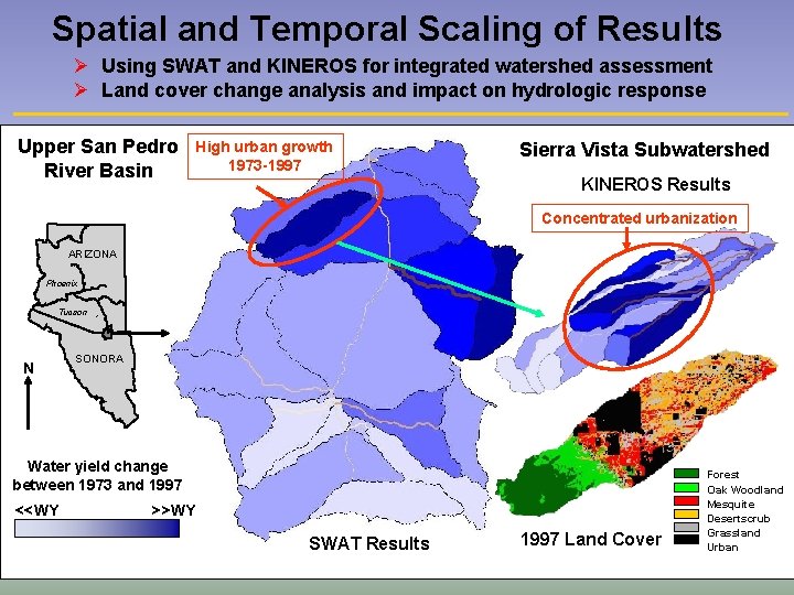
Spatial and Temporal Scaling of Results Ø Using SWAT and KINEROS for integrated watershed assessment Ø Land cover change analysis and impact on hydrologic response Upper San Pedro River Basin High urban growth 1973 -1997 Sierra Vista Subwatershed KINEROS Results Concentrated urbanization ARIZONA Phoenix # N # Tucson SONORA Water yield change between 1973 and 1997 <<WY >>WY SWAT Results 1997 Land Cover Forest Oak Woodland Mesquite Desertscrub Grassland Urban

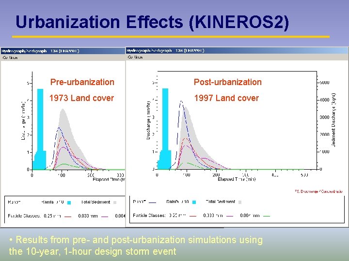
Urbanization Effects (KINEROS 2) Pre-urbanization Post-urbanization 1973 Land cover 1997 Land cover • Results from pre- and post-urbanization simulations using the 10 -year, 1 -hour design storm event

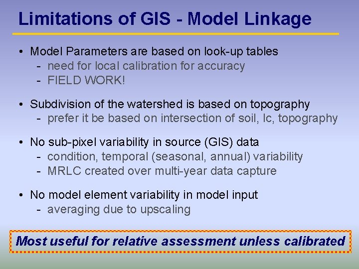
Limitations of GIS - Model Linkage • Model Parameters are based on look-up tables - need for local calibration for accuracy - FIELD WORK! • Subdivision of the watershed is based on topography - prefer it be based on intersection of soil, lc, topography • No sub-pixel variability in source (GIS) data - condition, temporal (seasonal, annual) variability - MRLC created over multi-year data capture • No model element variability in model input - averaging due to upscaling Most useful for relative assessment unless calibrated

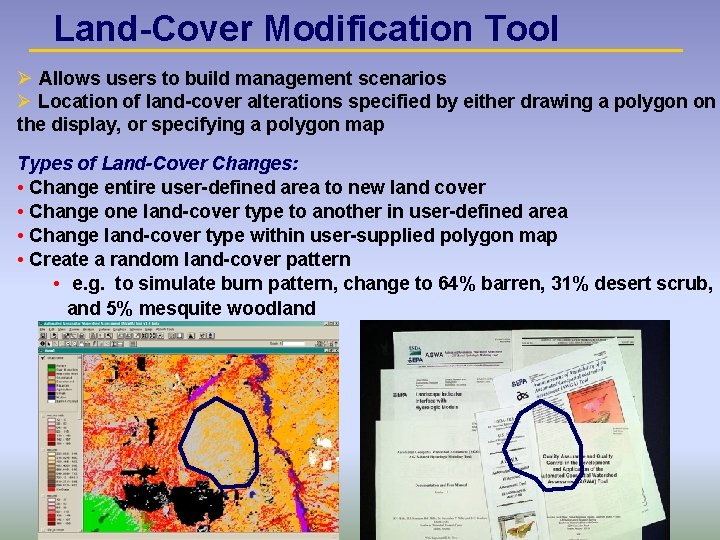
Land-Cover Modification Tool Ø Allows users to build management scenarios Ø Location of land-cover alterations specified by either drawing a polygon on the display, or specifying a polygon map Types of Land-Cover Changes: • Change entire user-defined area to new land cover • Change one land-cover type to another in user-defined area • Change land-cover type within user-supplied polygon map • Create a random land-cover pattern • e. g. to simulate burn pattern, change to 64% barren, 31% desert scrub, and 5% mesquite woodland

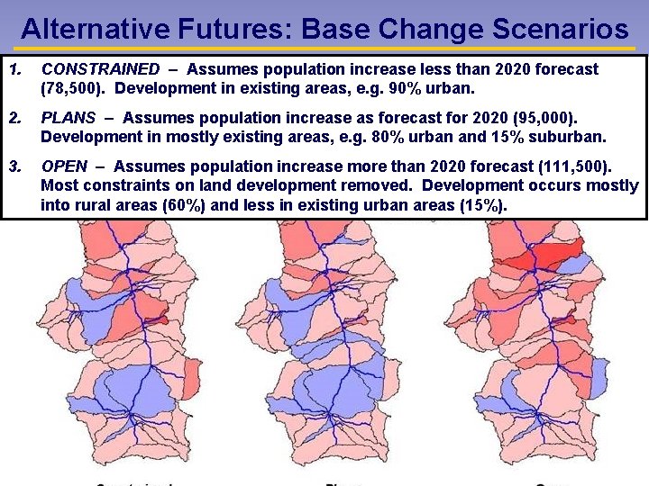
Alternative Futures: Base Change Scenarios 1. CONSTRAINED – Assumes population increase less than 2020 forecast (78, 500). Development in existing areas, e. g. 90% urban. 2. PLANS – Assumes population increase as forecast for 2020 (95, 000). Development in mostly existing areas, e. g. 80% urban and 15% suburban. 3. OPEN – Assumes population increase more than 2020 forecast (111, 500). Most constraints on land development removed. Development occurs mostly into rural areas (60%) and less in existing urban areas (15%).

Percent Change in Runoff under Future Scenarios • There is considerable variation – particularly between extremes produced by constrained and open scenarios (Kepner et al. , 2004) • Surface runoff will increase in all three scenarios • Sediment yield will increase especially as new surfaces are disturbed and surface runoff increases (Derived from using future land covers and AGWA)

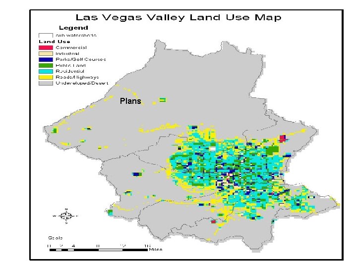
Plans

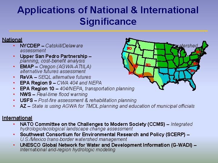
Applications of National & International Significance National • NYCDEP – Catskill/Delaware watershed assessment • Upper San Pedro Partnership – watershed planning, cost-benefit analysis • EMAP – Oregon (AGWA-ATt. ILA) integrated alternative futures assessment • Re. VA – SEQL alternative futures • EPA Region 9 – CWA 404 and NEPA • EPA Region 10 – 404/NEPA, transportation planning • NWS – Real-time flood warning • USFS – Post-fire assessment & rehabilitation planning • AZ – State is using AGWA for TMDL planning and education of municipal officials International • NATO Committee on the Challenges to Modern Society (CCMS) – Integrated hydrologic/ecological landscape change assessment • Southwest Consortium for Environmental Research and Policy (SCERP) – U. S. /Mexico trans-border watershed management • UNESCO Global Network for Water and Development Information (G-WADI) – International arid-region hydrologic modeling

AGWA Milestones • AGWA 1. 1 released at the Fed. Interagency Hydrologic Modeling Conference, July 2002 • Externally peer-evaluated through two separate federal review processes (EPA/600/R-02/046 & ARS/137460) • AGWA added to • • • EPA Council for Regulatory Environmental Modeling (CREM) database NASA Applied Sciences Directorate model and analysis systems USGS Surface-water Modeling Interest Group archives • • AGWA 1. 4 released in July, 2004 • • Training – national and international • 1200+ registered users (excluding BASINS users) AGWA integrated into BASINS 3. 1 release, August 2004 Free public download and full documentation via parallel EPA and ARS web sites

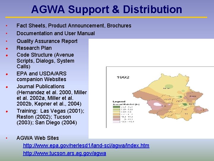
AGWA Support & Distribution • • • l l l • Fact Sheets, Product Announcement, Brochures Documentation and User Manual Quality Assurance Report Research Plan Code Structure (Avenue Scripts, Dialogs, System Calls) EPA and USDA/ARS companion Websites Journal Publications (Hernandez et al. 2000, Miller et al. 2002 a, Miller et al. 2002 b, Kepner et al. , 2004) Training: Las Vegas (2001); Reston (2002); Tucson (2003); San Diego (2004) AGWA Web Sites http: //www. epa. gov/nerlesd 1/land-sci/agwa/index. htm http: //www. tucson. ars. ag. gov/agwa

Future Directions Migrating to Arc. GIS (AGWA 2. 0) and the Internet (Dot. AGWA) • Final Arc. View version (AGWA 1. 5) release at FIHMC (April 2006) • Detailed, peer reviewed design plan for AGWA migration to Arc. GIS and Internet completed April, 2005 • Beta-release of Arc. GIS and Internet versions, 2006 • Final Arc. GIS and Internet release with full documentation, 2007 Integration of additional models • Opus – USDA-ARS integrated simulation model for transport of nonpoint source pollutants (2007) • MODFLOW – USGS ground-water model will be coupled with AGWAKINEROS surface-water model (planning meeting 2006) • GAP habitat models – integrated hydrologic and ecological assessments (proposal pending)