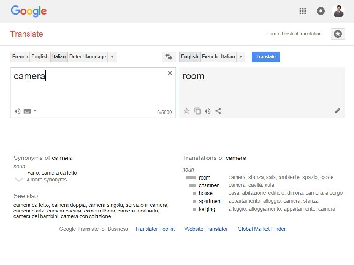
Camera model and calibration Samuel Cheng Slide credit

Camera model and calibration Samuel Cheng Slide credit: James Tompkin, Naoh Snavely

What is a camera?

Camera obscura: dark room • Known during classical period in China and Greece (e. g. , Mo-Ti, China, 470 BC to 390 BC) Illustration of Camera Obscura Freestanding camera obscura at UNC Chapel Hill Photo by Seth Ilys James Hays

Camera obscura / lucida used for tracing Lens Based Camera Obscura, 1568 Camera lucida drawingchamber. wordpress. com

First Photograph Oldest surviving photograph • Took 8 hours on pewter plate Joseph Niepce, 1826 Photograph of the first photograph Stored at UT Austin Niepce later teamed up with Daguerre, who eventually created Daguerrotypes
 3 D world 2 D image")
Dimensionality Reduction Machine (3 D to 2 D) 3 D world 2 D image Figures © Stephen E. Palmer, 2002

Holbein’s The Ambassadors - 1533

Holbein’s The Ambassadors – Memento Mori
 c")
Pinhole camera model d c Real object d = Focal length (or f) c = Optical center of the camera Figure from Forsyth
")
Modeling projection PP: projection plane COP: center of projection • Both (x’, y’, -d) and (x, y, z) project to the same point at PP • (x, y, z) -> (x’, y’) where x’ = d (x/z) and y’ = d (y/z)
 w Trick: add one more coordinate: homogeneous plane w")
Homogeneous coordinates (x, y, w) w Trick: add one more coordinate: homogeneous plane w = 1 (x/w, y/w, 1) x homogeneous image coordinates y Converting from homogeneous coordinates

Modeling projection • Is the projection a linear transformation? • no—division by z is nonlinear Homogeneous coordinates to the rescue! Recall that: homogeneous image coordinates homogeneous scene coordinates

Perspective Projection is a matrix multiply using homogeneous coordinates: divide by third coordinate This is known as perspective projection • The matrix is the projection matrix

Perspective Projection • Note that scaling the projection matrix does not change the transform

Perspective projection

Orthographic Projection • Special case of perspective projection • Distance from the COP to the image plane is infinite Image World • Also called “parallel projection” • What’s the projection matrix? Slide by Steve Seitz

Variants of orthographic projection • Scaled orthographic • Also called “weak perspective” • Affine projection • Also called “paraperspective”

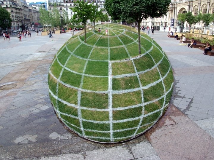
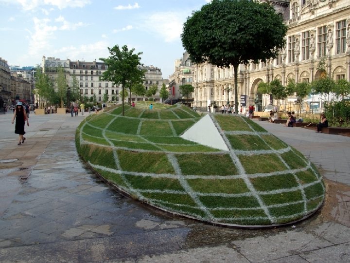
Perspective projection What is preserved? • Straight lines are still straight.

Vanishing points and lines Parallel lines in the world intersect in the projected image at a “vanishing point”. Parallel lines on the same plane in the world converge to vanishing points on a “vanishing line”. E. G. , the horizon. Vanishing Point Vanishing Line Vanishing Point

Vanishing points and lines Vanishing point Slide from Efros, Photo from Criminisi Vertical vanishing point (at infinity) Vanishing point

Projection properties • Many-to-one: any points along same ray map to same point in image • Points → points • Lines → lines • But line through focal point projects to a point • Planes → planes (or half-planes) • But plane through focal point projects to line

Camera parameters How many numbers do we need to describe a camera? • We need to describe its pose in the world • We need to describe its internal parameters

A Tale of Two Coordinate Systems v COP w y u Camera Two important coordinate systems: 1. World coordinate system 2. Camera coordinate system x o z “The World”
 in world coordinates into a")
Camera parameters To project a point (x, y, z) in world coordinates into a camera • First transform (x, y, z) into camera coordinates • Need to know extrinsics • Camera position (in world coordinates) • Camera orientation (in world coordinates) • Then project into the image plane • Need to know camera intrinsics • Coming soon • These can all be described with matrices

Extrinsics • How do we get the camera to “canonical form”? • (Center of projection at the origin, x-axis points right, y-axis points up, z-axis points backwards) Step 1: Translate by -c 0

Extrinsics • How do we get the camera to “canonical form”? • (Center of projection at the origin, x-axis points right, y-axis points up, z-axis points backwards) Step 1: Translate by -c How do we represent translation as a matrix multiplication? 0

Extrinsics • How do we get the camera to “canonical form”? • (Center of projection at the origin, x-axis points right, y-axis points up, z-axis points backwards) Step 1: Translate by -c Step 2: Rotate by R 0 3 x 3 rotation matrix

Extrinsics • How do we get the camera to “canonical form”? • (Center of projection at the origin, x-axis points right, y-axis points up, z-axis points backwards) Step 1: Translate by -c Step 2: Rotate by R 0

Camera parameters A camera is described by several parameters • • Translation T of the optical center from the origin of world coords Rotation R of the image plane focal length f, principle point (x’c, y’c), pixel size (sx, sy) blue parameters are called “extrinsics, ” red are “intrinsics” Projection equation • The projection matrix models the cumulative effect of all parameters • Useful to decompose into a series of operations identity matrix intrinsics projection rotation translation • The definitions of these parameters are not completely standardized – especially intrinsics—varies from one book to another
 matrix Slide Credit: Savarese R, t jw X kw Ow iw x")
Camera (projection) matrix Slide Credit: Savarese R, t jw X kw Ow iw x Extrinsic Matrix x: Image Coordinates: (U, V, 1) K: Intrinsic Matrix (3 x 3) R: Rotation (3 x 3) t: Translation (3 x 1) X: World Coordinates: (X, Y, Z, 1)
 di O’ x X (0, 0, 0) Intrinsic Assumptions •")
Projection matrix (ignore extrinsics) di O’ x X (0, 0, 0) Intrinsic Assumptions • Unit aspect ratio • Optical center at (0, 0) • No skew Slide Credit: Savarese Extrinsic Assumptions • No rotation • Camera at (0, 0, 0) K
 Intrinsic")
Remove assumption: aligned optical center di X O’ O’ x (0, 0, 0) Intrinsic Assumptions • Unit aspect ratio • Optical center at -(U 0, V 0) • No skew Slide Credit: Savarese Extrinsic Assumptions • No rotation • Camera at (0, 0, 0) K
 Intrinsic")
Remove assumption: aligned optical center di X O’ O’ x (0, 0, 0) Intrinsic Assumptions • Unit aspect ratio • Optical center at -(U 0, V 0) • No skew Slide Credit: Savarese Extrinsic Assumptions • No rotation • Camera at (0, 0, 0) K
 Intrinsic")
Remove assumption: unit aspect ratio di X O’ O’ x (0, 0, 0) Intrinsic Assumptions • Optical center at -(U 0, V 0) • No skew Extrinsic Assumptions • No rotation • Camera at (0, 0, 0) K Slide Credit: Savarese
 Intrinsic Assumptions")
Remove assumption: non-skewed pixels di X O’ O’ x (0, 0, 0) Intrinsic Assumptions • Optical center at -(U 0, V 0) Extrinsic Assumptions • No rotation • Camera at (0, 0, 0) K Slide Credit: Savarese

Summary James Hays

Camera Matrix DEMO

Beyond Pinholes: Radial Distortion Radial distortion can be introduced due to the use of lens . . . Corrected Barrel Distortion Image from Martin Habbecke

Radial distortion • Radial distortion can be reduced by the following correction • r is the radial distance from the center of the scene • The parameters can be estimated by shooting straight lines since a straight line is supposed to be preserved under perspective projection

World vs Camera coordinates James Hays

James Hays Calibrating the Camera Use an scene with known geometry • Correspond image points to 3 d points • Get least squares solution (or non-linear solution) Known 3 d Known 2 d world locations image coords M Unknown Camera Parameters

How do we calibrate a camera? Known 2 d image coords Known 3 d world locations 880 214 43 203 270 197 886 347 745 302 943 128 476 590 419 214 317 335 783 521 235 427 665 429 655 362 427 333 412 415 746 351 434 415 525 234 716 308 602 187 312. 747 309. 140 30. 086 305. 796 311. 649 30. 356 307. 694 312. 358 30. 418 310. 149 307. 186 29. 298 311. 937 310. 105 29. 216 311. 202 307. 572 30. 682 307. 106 306. 876 28. 660 309. 317 312. 490 30. 230 307. 435 310. 151 29. 318 308. 253 306. 300 28. 881 306. 650 309. 301 28. 905 308. 069 306. 831 29. 189 309. 671 308. 834 29. 029 308. 255 309. 955 29. 267 307. 546 308. 613 28. 963 311. 036 309. 206 28. 913 307. 518 308. 175 29. 069 309. 950 311. 262 29. 990 312. 160 310. 772 29. 080 311. 988 312. 709 30. 514 James Hays

Unknown Camera Parameters Known 2 d image coords Known 3 d locations First, work out where X, Y, Z projects to under candidate M. Two equations per 3 D point correspondence James Hays

Unknown Camera Parameters Known 2 d image coords Next, rearrange into form where all M coefficients are individually stated in terms of X, Y, Z, u, v. -> Allows us to form lsq matrix. Known 3 d locations

Unknown Camera Parameters Known 2 d image coords Next, rearrange into form where all M coefficients are individually stated in terms of X, Y, Z, u, v. -> Allows us to form lsq matrix. Known 3 d locations

Unknown Camera Parameters Known 2 d image coords Known 3 d locations • Finally, solve for m’s entries using linear least squares Ax=b form • Method 1 – James Hays

Least squares • Find x that minimizes

Unknown Camera Parameters Known 2 d image coords Known 3 d locations • Finally, solve for m’s entries using linear least squares Ax=b form • Method 1 – x = Ab; x = [x; 1]; M = reshape(x, 4, 3)'; James Hays

Unknown Camera Parameters Known 2 d image coords Known 3 d locations • Or, solve for m’s entries using total linear least-squares. • Method 2 – Ax=0 form James Hays

Ax=0 • Note that x=0 is a trivial solution and has to be avoided • Consider instead

SVD and eigen-decomposition • Need to solve the eigen-decomposition problem of ATA. But often it is better to solve SVD of A instead • SVD: Singular value decomposition • Every real matrix A can be written as USVT, where U and V are orthogonal and S is diagonal • Consider ATA=(VSUT)USVT=VS 2 VT • That is, (ATA)V=VS 2, V is eigenvector matrix of ATA and S 2 is eigenvalue matrix of ATA • Instead of solving eigen-decomposition of ATA, we can solve SVD of A instead

Unknown Camera Parameters Known 2 d image coords Known 3 d locations • Or, solve for m’s entries using total linear least-squares. • Method 2 – Ax=0 form [U, S, V] = svd(A); x = V(: , end); M = reshape(x, 4, 3)'; James Hays

How do we calibrate a camera? Known 2 d image coords Known 3 d world locations 880 214 43 203 270 197 886 347 745 302 943 128 476 590 419 214 317 335 783 521 235 427 665 429 655 362 427 333 412 415 746 351 434 415 525 234 716 308 602 187 312. 747 309. 140 30. 086 305. 796 311. 649 30. 356 307. 694 312. 358 30. 418 310. 149 307. 186 29. 298 311. 937 310. 105 29. 216 311. 202 307. 572 30. 682 307. 106 306. 876 28. 660 309. 317 312. 490 30. 230 307. 435 310. 151 29. 318 308. 253 306. 300 28. 881 306. 650 309. 301 28. 905 308. 069 306. 831 29. 189 309. 671 308. 834 29. 029 308. 255 309. 955 29. 267 307. 546 308. 613 28. 963 311. 036 309. 206 28. 913 307. 518 308. 175 29. 069 309. 950 311. 262 29. 990 312. 160 310. 772 29. 080 311. 988 312. 709 30. 514 James Hays

Known 2 d image coords 1 st point 880 214 43 203 270 197 886 347 745 302 943 128 476 590 419 214 317 335 … Known 3 d world locations 312. 747 309. 140 30. 086 305. 796 311. 649 30. 356 307. 694 312. 358 30. 418 310. 149 307. 186 29. 298 311. 937 310. 105 29. 216 311. 202 307. 572 30. 682 307. 106 306. 876 28. 660 309. 317 312. 490 30. 230 307. 435 310. 151 29. 318 …. . Projection error defined by two equations – one for u and one for v

Known 2 d image coords 2 nd point 880 214 43 203 270 197 886 347 745 302 943 128 476 590 419 214 317 335 … Known 3 d world locations 312. 747 309. 140 30. 086 305. 796 311. 649 30. 356 307. 694 312. 358 30. 418 310. 149 307. 186 29. 298 311. 937 310. 105 29. 216 311. 202 307. 572 30. 682 307. 106 306. 876 28. 660 309. 317 312. 490 30. 230 307. 435 310. 151 29. 318 …. . Projection error defined by two equations – one for u and one for v

How many points do I need to fit the model? Degrees of freedom? 5 6 Think 3: - Rotation around x - Rotation around y - Rotation around z

How many points do I need to fit the model? Degrees of freedom? 5 6 M is 3 x 4, so 12 unknowns, but projective scale ambiguity – 11 deg. freedom. One equation per unknown -> 5 1/2 point correspondences determines a solution (e. g. , either u or v). More than 5 1/2 point correspondences -> overdetermined, many solutions to M. Least squares is finding the solution that best satisfies the overdetermined system. Why use more than 6? Robustness to error in feature points.

Summary
![Can we factorize M back to K [R | t]? • Yes! • We](http://slidetodoc.com/presentation_image_h/c463f0aaff0693a389d28955a5310561/image-62.jpg "Can we factorize M back to K [R | t]? • Yes! • We")
Can we factorize M back to K [R | t]? • Yes! • We can directly solve for the individual entries of K [R | t]. James Hays
![Can we factorize M back to K [R | t]? • Yes! • We](http://slidetodoc.com/presentation_image_h/c463f0aaff0693a389d28955a5310561/image-63.jpg "Can we factorize M back to K [R | t]? • Yes! • We")
Can we factorize M back to K [R | t]? • Yes! • We can also use RQ factorization (not QR) • R in RQ is not rotation matrix R; crossed names! • R (right diagonal) is K • Q (orthogonal basis) is R. • t, the last column of [R | t], is inv(K) * last column of M. • See http: //ksimek. github. io/2012/08/14/decompose/ for more details James Hays

Recovering the camera center t m 4 t= K-1 m 4 T=R-1 t=R-1 K-1 m 4 Q James Hays

Estimate of camera center 1. 0486 -0. 3645 -1. 6851 -0. 4004 -0. 9437 -0. 4200 1. 0682 0. 0699 0. 6077 -0. 0771 1. 2543 -0. 6454 -0. 2709 0. 8635 -0. 4571 -0. 3645 -0. 7902 0. 0307 0. 7318 0. 6382 -1. 0580 0. 3312 0. 3464 0. 3377 0. 3137 0. 1189 -0. 4310 0. 0242 -0. 4799 0. 2920 0. 6109 0. 0830 -0. 4081 0. 2920 -0. 1109 -0. 2992 0. 5129 -0. 0575 0. 1406 -0. 4527 1. 5706 -0. 1490 0. 2598 -1. 5282 0. 9695 0. 3802 -0. 6821 1. 2856 0. 4078 0. 4124 -1. 0201 -0. 0915 1. 2095 0. 2812 -0. 1280 0. 8819 -0. 8481 0. 5255 -0. 9442 -1. 1583 -0. 3759 0. 0415 1. 3445 0. 3240 -0. 7975 0. 3017 -0. 0826 -0. 4329 -1. 4151 -0. 2774 -1. 1475 -0. 0772 -0. 2667 -0. 5149 -1. 1784 -0. 1401 0. 1993 -0. 2854 -0. 2114 -0. 4320 0. 2143 -0. 1053 -0. 7481 -0. 3840 -0. 2408 0. 8078 -0. 1196 -0. 2631 -0. 7605 -0. 5792 -0. 1936 0. 3237 0. 7970 0. 2170 1. 3089 0. 5786 -0. 1887 1. 2323 1. 4421 0. 4506

Calibration with non-linear methods • Linear calibration • Advantages • Easy to formulate and solve • Provides initialization for non-linear methods • Disadvantages • Doesn’t directly give you camera parameters • Doesn’t model radial distortion • Can’t impose constraints, such as known focal length • Non-linear calibrations • Define error as difference between projected points and measured points • Minimize error using Newton’s method or other non-linear optimization James Hays

Open. CV Calibration Demo
- Slides: 67