Author Saeed Shiry With little change by Keyvanrad

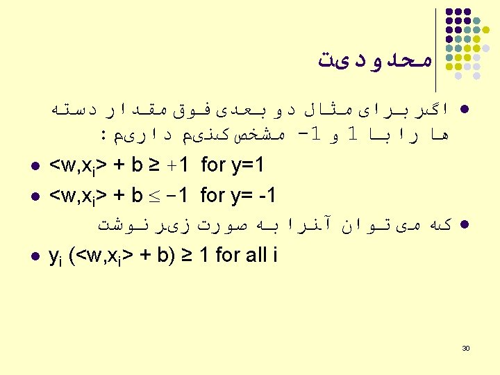
ﻣﺎﺷیﻦ ﺑﺮﺩﺍﺭ پﺸﺘیﺒﺎﻥ Author : Saeed Shiry With little change by: Keyvanrad 1 1393 -1394 (Spring)
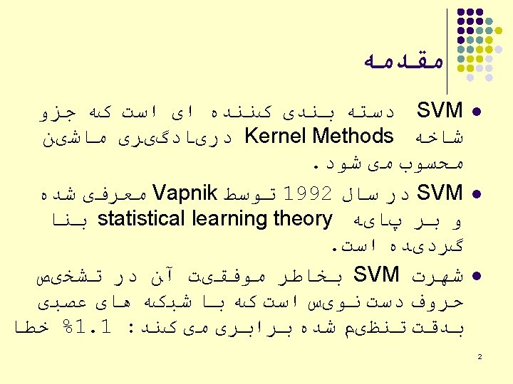


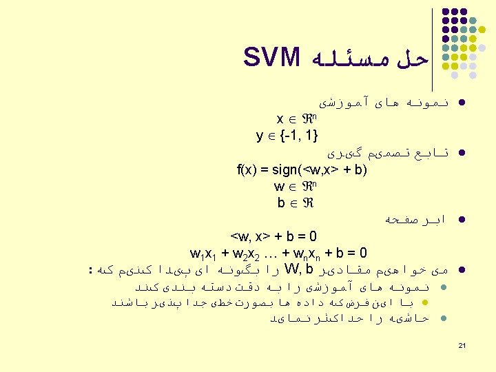
ﺗﻌﺮیﻒ l Support Vector Machines are a system for efficiently training linear learning machines in kernel-induced feature spaces, while respecting the insights of generalisation theory and exploiting optimisation theory. l Cristianini & Shawe-Taylor (2000) 4

Intuitions X X X O X O O O 6

Intuitions X X X O X O O O 7

Intuitions X X X O X O O O 8

Intuitions X X X O X O O O 9

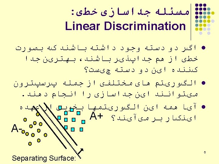
A “Good” Separator X X X O X O O O 10

Noise in the Observations X X X O X O O O 11

Ruling Out Some Separators X X X O X O O O 12

Lots of Noise X X X O X O O O 13

Maximizing the Margin X X X O X O O O 14
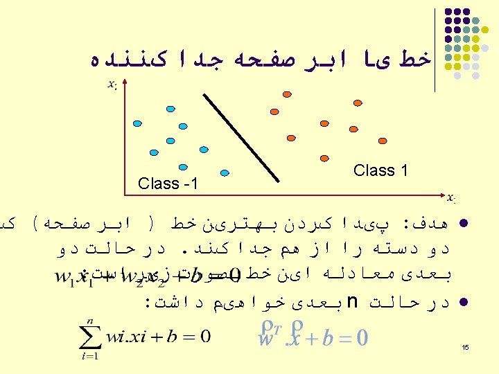
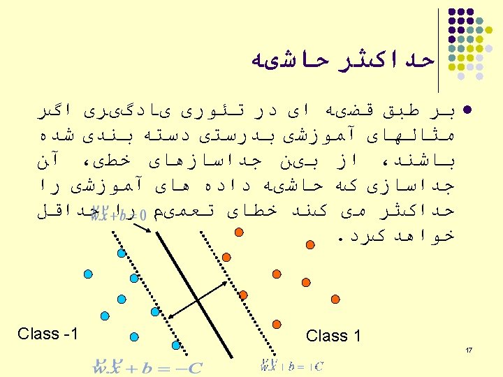

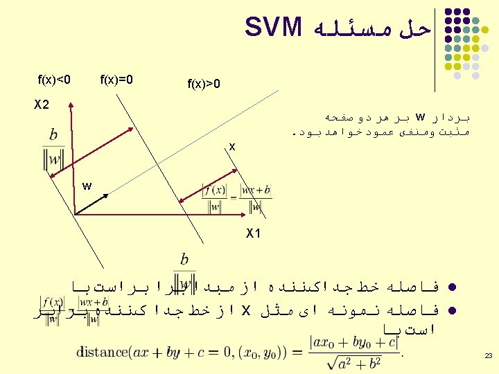
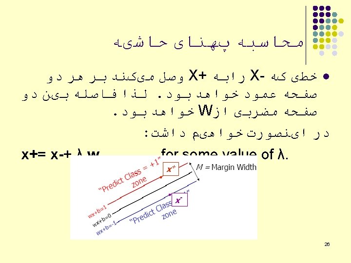
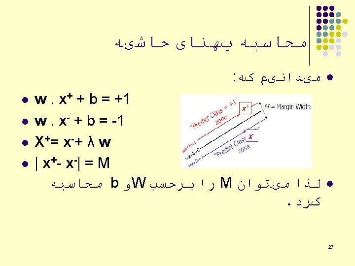
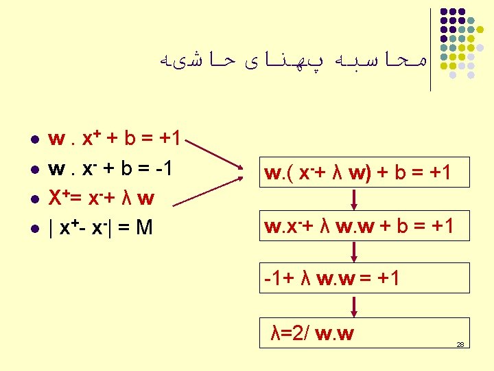
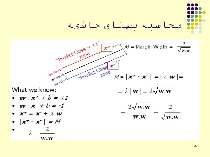
Linear SVM Mathematically l w. Txi + b ≤ - ρ/2 if yi = -1 w. Txi + b ≥ ρ/2 if yi = 1 yi(w. Txi + b) ≥ ρ/2 22
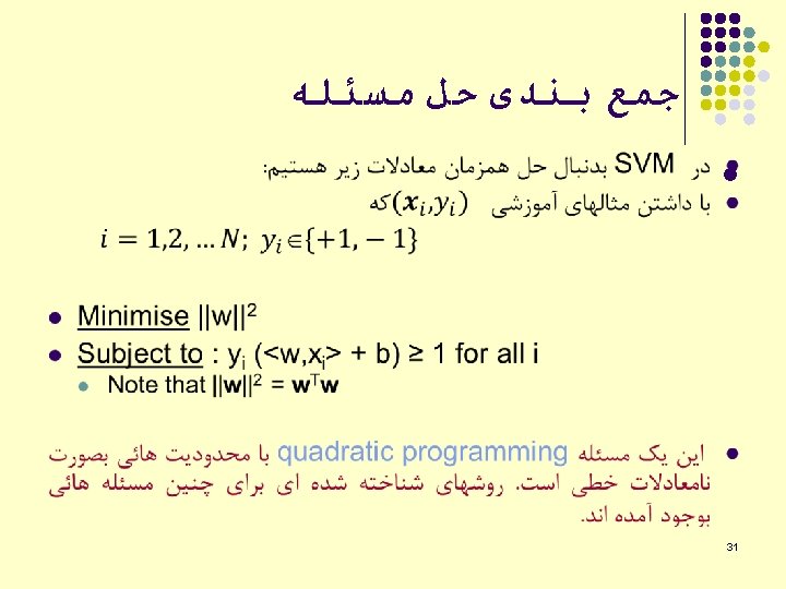

Quadratic Programming 32
 subject to")
Recap of Constrained Optimization l l Suppose we want to: minimize f(x) subject to g(x) = 0 A necessary condition for x 0 to be a solution: : the Lagrange multiplier For multiple constraints gi(x) = 0, i=1, …, m, we need a Lagrange multiplier i for each of the constraints 33
 £ 0 is")
Recap of Constrained Optimization l The case for inequality constraint gi(x) £ 0 is similar, except that the Lagrange multiplier i should be positive If x 0 is a solution to the constrained optimization problem l There must exist i ≥ 0 for i=1, …, m such that x 0 satisfy l The function l is also known as the Lagrangrian; we want to set its gradient to 0 34

ﺭﺍﻩ ﺣﻞ ﻣﻌﺎﺩﻟﻪ l Construct & minimise the Lagrangian l Take derivatives wrt. w and b, equate them to 0 parameters are expressed as a linear combination of training points only SVs will have non-zero i The Lagrange multipliers i are called ‘dual variables’ Each training point has an associated dual variable. 35

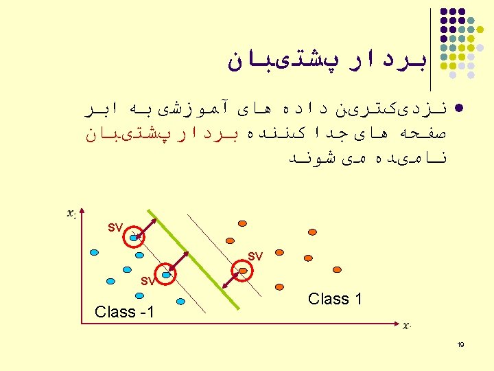
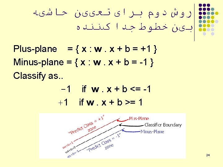
ﺭﺍﻩ ﺣﻞ ﻣﻌﺎﺩﻟﻪ Class 2 8=0. 6 10=0 7=0 5=0 4=0 9=0 Class 1 2=0 1=0. 8 6=1. 4 3=0 36

The Dual Problem l If we substitute l Note that l This is a function of i only to Lagrangian , we have 37

The Dual Problem l l l The new objective function is in terms of i only It is known as the dual problem: if we know w, we know all i; if we know all i, we know w The original problem is known as the primal problem The objective function of the dual problem needs to be maximized! The dual problem is therefore: Properties of i when we introduce the Lagrange multipliers The result when we differentiate the original Lagrangian w. r. t. b 38
 problem l l A")
The Dual Problem l This is a quadratic programming (QP) problem l l A global maximum of i can always be found w can be recovered by 39

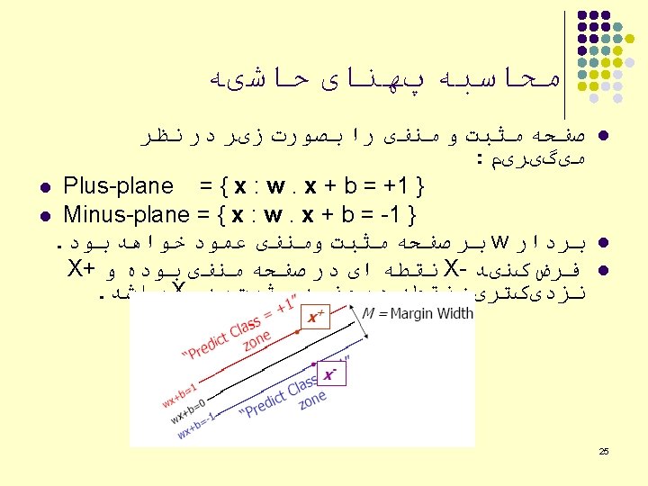
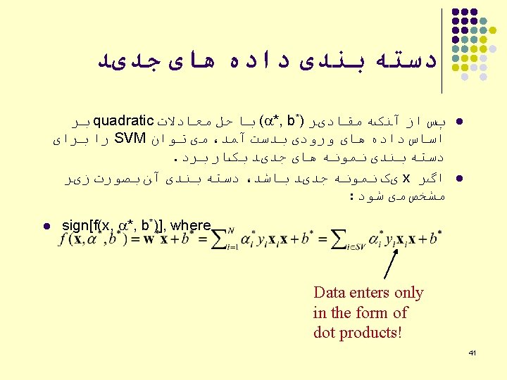
ﺭﺍﻩ ﺣﻞ ﻣﻌﺎﺩﻟﻪ l l So, Plug this back into the Lagrangian to obtain the dual formulation The resulting dual that is solved for by using a QP solver: The b does not appear in the dual so it is determined separately from the initial constraints Data enters only in the form of dot products! 40

ﻭیژگی ﻫﺎی ﺭﺍﻩ ﺣﻞ l l l The solution of the SVM, i. e. of the quadratic programming problem with linear inequality constraints has the nice property that the data enters only in the form of dot products! Dot product (notation & memory refreshing): given x=(x 1, x 2, …xn) and y=(y 1, y 2, …yn), then the dot product of x and y is xy=(x 1 y 1, x 2 y 2, …, xnyn). This is nice because it allows us to make SVMs nonlinear without complicating the algorithm 42

The Quadratic Programming Problem l l Many approaches have been proposed l Loqo, cplex, etc. Most are “interior-point” methods l Start with an initial solution that can violate the constraints l Improve this solution by optimizing the objective function and/or reducing the amount of constraint violation For SVM, sequential minimal optimization (SMO) seems to be the most popular l A QP with two variables is trivial to solve l Each iteration of SMO picks a pair of ( i, j) and solve the QP with these two variables; repeat until convergence In practice, we can just regard the QP solver as a “black-box” without bothering how it works 43
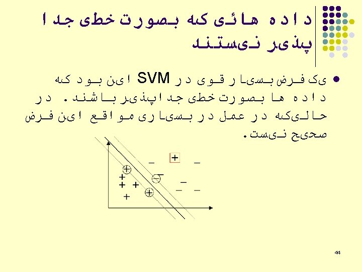
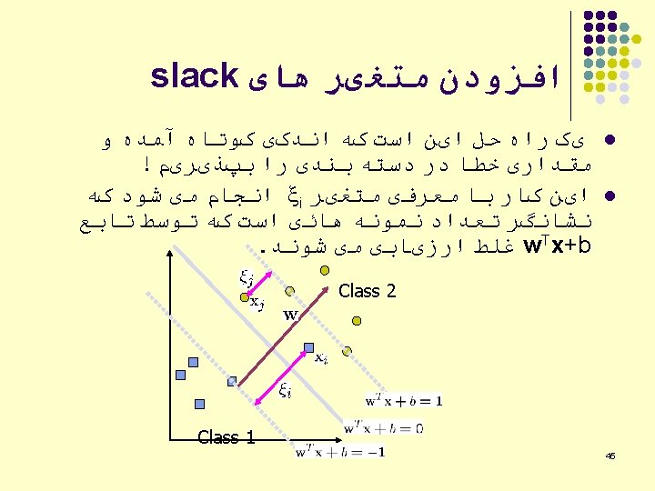

Soft Margin Hyperplane l If we minimize wi xi, xi can be computed by l xi are “slack variables” in optimization l l l We want to minimize l l Note that xi=0 if there is no error for xi xi is an upper bound of the number of errors C : tradeoff parameter between error and margin The optimization problem becomes 49

The Optimization Problem l The dual of this new constrained optimization problem is l w is recovered as l This is very similar to the optimization problem in the linear separable case, except that there is an upper bound C on i now Once again, a QP solver can be used to find i l 50

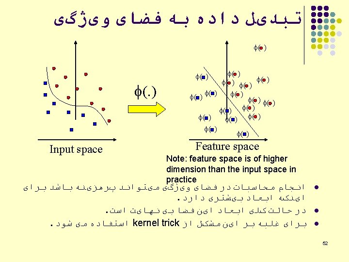


ﻧگﺎﺷﺖ ﻏیﺮ ﻣﺴﺘﻘیﻢ ﺑﻪ ﻓﻀﺎی ﻭیژگی l We will introduce Kernels: l l Solve the computational problem of working with many dimensions Can make it possible to use infinite dimensions efficiently in time / space Other advantages, both practical and conceptual 54
 The linear algorithm depends only on")
کﺮﻧﻞ l l l Transform x (x) The linear algorithm depends only on xxi, hence transformed algorithm depends only on (x) (xi) Use kernel function K(xi, xj) such that K(xi, xj)= (x) (xi) 55
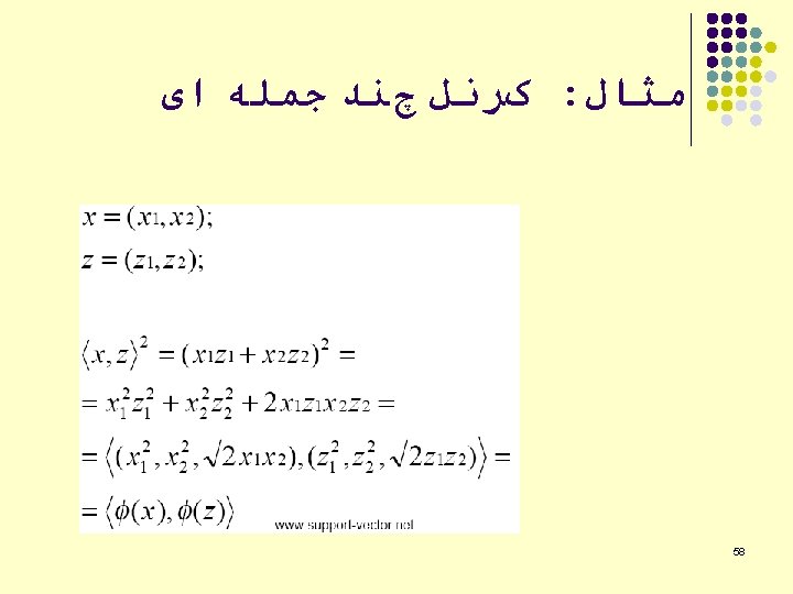
 and K(. , . ) l Suppose (. )")
An Example for f(. ) and K(. , . ) l Suppose (. ) is given as follows l An inner product in the feature space is l So, if we define the kernel function as follows, there is no need to carry out (. ) explicitly l This use of kernel function to avoid carrying out (. ) explicitly is known as the kernel trick 56
 57")
: کﺮﻧﻞ ﻫﺎی ﻧﻤﻮﻧﻪ Homogeneous Polynomial Kernel (C=0) 57

Modification Due to Kernel Function l l Change all inner products to kernel functions For training, Original With kernel function 59

Modification Due to Kernel Function l For testing, the new data z is classified as class 1 if f³ 0, and as class 2 if f <0 Original With kernel function 60

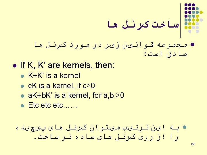
Modularity l Any kernel-based learning algorithm composed of two modules: l l l A general purpose learning machine A problem specific kernel function Any K-B algorithm can be fitted with any kernel Kernels themselves can be constructed in a modular way Great for software engineering (and for analysis) 61

Example l l l Suppose we have 5 1 D data points l x 1=1, x 2=2, x 3=4, x 4=5, x 5=6, with 1, 2, 6 as class 1 and 4, 5 as class 2 y 1=1, y 2=1, y 3=-1, y 4=-1, y 5=1 We use the polynomial kernel of degree 2 l K(x, z) = (xz+1)2 l C is set to 100 We first find i (i=1, …, 5) by 63

Example l By using a QP solver, we get l l l 1=0, 2=2. 5, 3=0, 4=7. 333, 5=4. 833 Note that the constraints are indeed satisfied The support vectors are {x 2=2, x 4=5, x 5=6} l The discriminant function is l b is recovered by solving f(2)=1 or by f(5)=-1 or by f(6)=1, as x 2 and x 5 lie on the line and x 4 lies on the line All three give b=9 l 64

Example Value of discriminant function class 1 class 2 1 2 4 5 6 65


ﺑﺮﺍی ﺩﺳﺘﻪ ﺑﻨﺪی SVM ﻣﺮﺍﺣﻞ ﺍﺳﺘﻔﺎﺩﻩ ﺍﺯ l l Prepare the data matrix Select the kernel function to use Execute the training algorithm using a QP solver to obtain the i values Unseen data can be classified using the i values and the support vectors 67

ﺍﻧﺘﺨﺎﺏ ﺗﺎﺑﻊ کﺮﻧﻞ l l l ﺍﻧﺘﺨﺎﺏ ﺗﺎﺑﻊ کﺮﻧﻞ SVM ﺟﺪی ﺗﺮیﻦ ﻣﺴﺌﻠﻪ ﺩﺭ ﺭﻭﺵ . ﺍﺳﺖ ﺭﻭﺷﻬﺎ ﻭ ﺍﺻﻮﻝ ﻣﺘﻌﺪﺩی ﺑﺮﺍی ﺍیﻦ کﺎﺭ ﻣﻌﺮﻓی ﺷﺪﻩ : ﺍﺳـﺖ diffusion kernel, Fisher kernel, string kernel, … ﻭ ﺗﺤﻘیﻘﺎﺗی ﻧیﺰ ﺑﺮﺍی ﺑﺪﺳﺖ آﻮﺭﺩﻥ ﻣﺎﺗﺮیﺲ کﺮﻧﻞ . ﺍﺯ ﺭﻭی ﺩﺍﺩﻩ ﻫﺎی ﻣﻮﺟﻮﺩ ﺩﺭ ﺣﺎﻝ ﺍﻧﺠﺎﻡ ﺍﺳﺖ ﺩﺭ ﻋﻤﻞ In practice, a low degree polynomial kernel or RBF kernel with a reasonable width is a good initial try Note that SVM with RBF kernel is closely related to RBF neural networks, with the centers of the radial basis functions automatically chosen for SVM l l 68

SVM applications l l l SVMs were originally proposed by Boser, Guyon and Vapnik in 1992 and gained increasing popularity in late 1990 s. SVMs are currently among the best performers for a number of classification tasks ranging from text to genomic data. SVMs can be applied to complex data types beyond feature vectors (e. g. graphs, sequences, relational data) by designing kernel functions for such data. SVM techniques have been extended to a number of tasks such as regression [Vapnik et al. ’ 97], principal component analysis [Schölkopf et al. ’ 99], etc. Most popular optimization algorithms for SVMs use decomposition to hill-climb over a subset of αi’s at a time, e. g. SMO [Platt ’ 99] and [Joachims ’ 99] Tuning SVMs remains a black art: selecting a specific kernel and parameters is usually done in a try-and-see manner. 69

SVM ﻧﻘﺎﻁ ﻗﻮﺕ ﻭ ﺿﻌﻒ l Strengths l l l l Training is relatively easy Good generalization in theory and practice Work well with few training instances Find globally best model, No local optimal, unlike in neural networks It scales relatively well to high dimensional data Tradeoff between classifier complexity and error can be controlled explicitly Weaknesses l Need to choose a “good” kernel function. 70

ﻧﺘیﺠﻪ گیﺮی l SVMs find optimal linear separator l l l They pick the hyperplane that maximises the margin The optimal hyperplane turns out to be a linear combination of support vectors The kernel trick makes SVMs non-linear learning algorithms l Transform nonlinear problems to higher dimensional space using kernel functions; then there is more chance that in the transformed space the classes will be linearly separable. 71

SVM ﺳﺎیﺮ ﺟﻨﺒﻪ ﻫﺎی l How to use SVM for multi-classification? l l How to interpret the SVM discriminant function value as probability? l l One can change the QP formulation to become multi-class More often, multiple binary classifiers are combined One can train multiple one-versus-all classifiers, or combine multiple pairwise classifiers “intelligently” By performing logistic regression on the SVM output of a set of data (validation set) that is not used for training Some SVM software (like libsvm) have these features built-in 72
![ﻣﺮﺍﺟﻊ [1] b. E. Boser et al. A training algorithm for optimal margin](http://slidetodoc.com/presentation_image_h2/39116b58d20b850903478af05bf0acd1/image-74.jpg "ﻣﺮﺍﺟﻊ [1] b. E. Boser et al. A training algorithm for optimal margin")
ﻣﺮﺍﺟﻊ [1] b. E. Boser et al. A training algorithm for optimal margin classifiers. Proceedings of the fifth annual workshop on computational learning theory 5 144 -152, Pittsburgh, 1992. [2] l. Bottou et al. Comparison of classifier methods: a case study in handwritten digit recognition. Proceedings of the 12 th IAPR international conference on pattern recognition, vol. 2, pp. 77 -82. [3] v. Vapnik. The nature of statistical learning theory. 2 nd edition, Springer, 1999. 74
- Slides: 74