Mixture of Experts Instructor Saeed Shiry 1 l

Mixture of Experts Instructor : Saeed Shiry 1

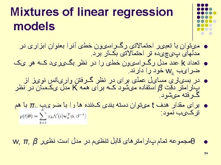
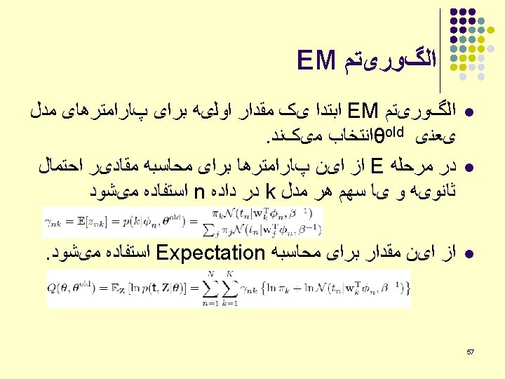
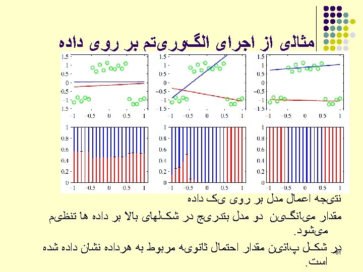
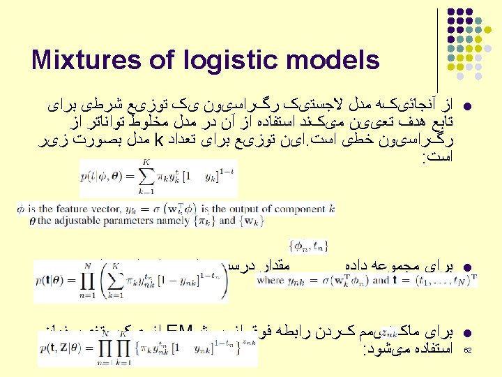
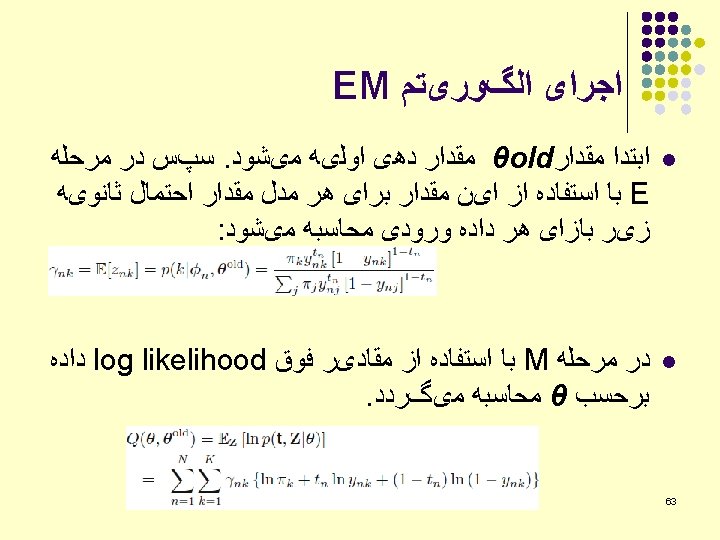
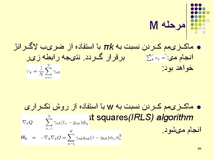
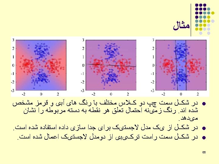
ﺭﻭﺵ l l l . ﺳﻪ ﺭﻭﺵ ﺩﺭ ﺍﺩﺍﻣﻪ ﻣﻮﺭﺩ ﺑﺤﺚ ﻗﺮﺍﺭ ﺧﻮﺍﻫﻨﺪ گﺮﻓﺖ Mixtures of linear regression models Mixtures of logistic regression models Mixture of experts model l 3

ﻣﺜﺎﻝ Suppose the following are marks in a course 55. 5, 67, 87, 48, 63 Marks typically follow a Normal distribution whose density function is Now, we want to find the best , such that

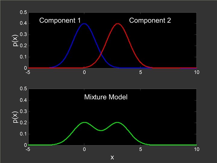
ﻣﺜﺎﻝ l Suppose we have data about heights of people (in cm) l l 185, 140, 134, 150, 170 Heights follow a normal (log normal) distribution but men on average are taller than women. This suggests a mixture of two distributions

A Mixture Distribution

Example of MLE Now, choose p which maximizes L(p). Instead we will maximize l(p)= Log. L(p) l

Two Important Facts l If A 1, , An are independent then l The log function is monotonically increasing. x · y ! Log(x) · Log(y) l Therefore if a function f(x) >= 0, achieves a maximum at x 1, then log(f(x)) also achieves a maximum at x 1.

Properties of MLE l There are several technical properties of the estimator but lets look at the most intuitive one: l As the number of data points increase we become more sure about the parameter p

Properties of MLE r is the number of data points. As the number of data points increase the confidence of the estimator increases.

Matlab commands [phat, ci]=mle(Data, ’distribution’, ’Bernoulli’); l [phi, ci]=mle(Data, ’distribution’, ’Normal’); l

ﺭﺍﻩ ﺣﻞ ﻣﺴﺌﻠﻪ l Problem: Describe data with Mixture Model(MM) l Approach: l Decide on MM, e. g. l l l Gauss distribution Mix of two Estimate parameters

Gaussian Mixture Model (GMM) l Assume that the dataset is generated by two mixed Gaussian distributions l l Gaussian model 1: Gaussian model 2: If we know the memberships for each bin, estimating the two Gaussian models is easy. How to estimate the two Gaussian models without knowing the memberships of bins?

Review l Stochastically independent l Bayes’ rule l Logarithm l Expectation

Types of classification data K-means: Data set is incomplete, but we complete it using a specific Data set is complete. cost function. EM: data set is incomplete, but we complete it using posterior probabilities (a “soft” class membership).

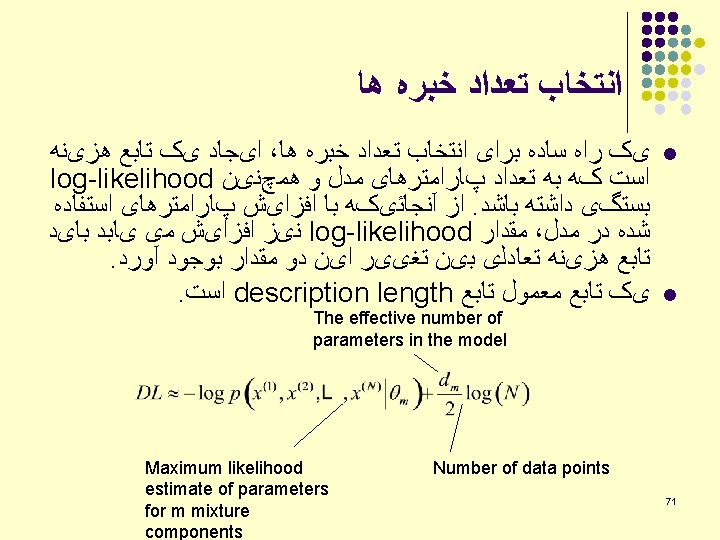
Motivation l Likelihood of parameter Θ given data X: l Maximize expectation of L by tweaking Θ: l l Analytically hard Use “Expectation Maximization” method and algorithm A. P. Dempster, et al 1977: “Maximum likelihood from incomplete data via the EM algorithm” Ø Ø Ø General statement of the algorithm Prove convergence Coin the term ”EM algorithm”

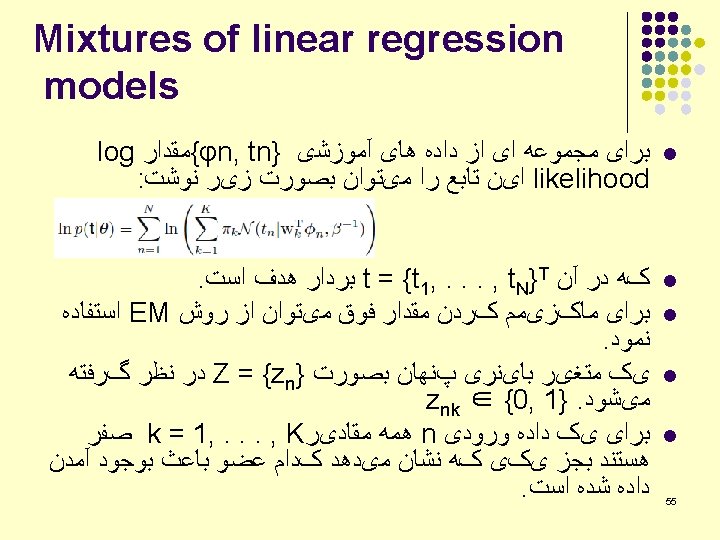
EM as A Bound Optimization l EM algorithm in fact maximizes the log-likelihood function of training data Likelihood for a data point x l Log-likelihood of training data l

EM as A Bound Optimization l EM algorithm in fact maximizes the log-likelihood function of training data Likelihood for a data point x l Log-likelihood of training data l

EM as A Bound Optimization l l EM algorithm in fact maximizes the log-likelihood function of training data Likelihood for a data point x p 1 = p( 1) = p(z 1 = 1) and p 2 = p( 2) = p(z 2 =1) 1=(µ 1, 1) and 2=(µ 2, 2)

Data Likelihood Remember: We have unlabeled data X = {x 1 x 2 … x. R} We know there are k classes We know P( 1) P( 2) P( 3) … P( k) We don’t know μ 1 μ 2. . μk We can write P( X | μ 1…. μk) = P( data | μ 1…. μk)

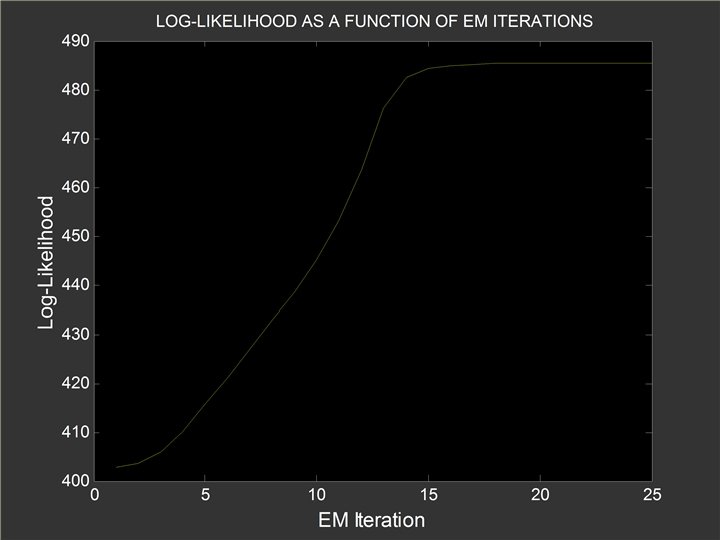
EM algorithm: log-likelihood increases with each step -870 -880 -890 -900 -910 -920 -930 0 10 20 30 40

Maximize GMM Model

The simplest data to model: a set of 1–d samples

Fit this distribution with a Gaussian

How find the parameters of the best-fitting Gaussian? Posterior probability Likelihood function mean data points std. dev. By Bayes rule Evidence Prior probability

How find the parameters of the best-fitting Gaussian? Posterior probability Likelihood function mean data points std. dev. Prior probability Evidence Maximum likelihood parameter estimation:

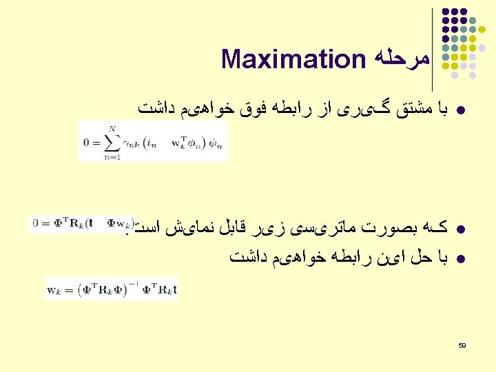
Derivation of MLE for Gaussians Observation density Log likelihood Maximisation

Basic Maximum Likelihood Estimate (MLE) of a Gaussian distribution Mean Variance Covariance Matrix

Basic Maximum Likelihood Estimate (MLE) of a Gaussian distribution Mean Variance For vector-valued data, we have the Covariance Matrix

EM Algorithm for GMM l Let memberships to be hidden variables l EM algorithm for Gaussian mixture model l Unknown memberships: l Unknown Gaussian models: l Learn these two sets of parameters iteratively

Start with A Random Guess l Random assign the memberships to each point

Start with A Random Guess l l Random assign the memberships to each point Estimate the means and variance of each Gaussian model

E-step l l Fixed the two Gaussian models Estimate the posterior for each data point

EM Algorithm for GMM Re-estimate the l memberships for each point

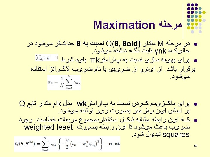
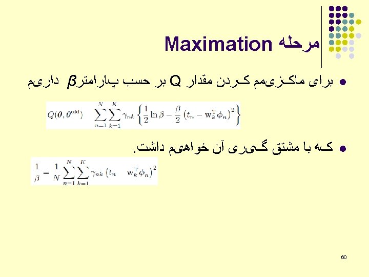
M-Step l l Fixed the memberships Re-estimate the two model Gaussian Q

EM Algorithm for GMM l l Re-estimate the memberships for each point Re-estimate the models

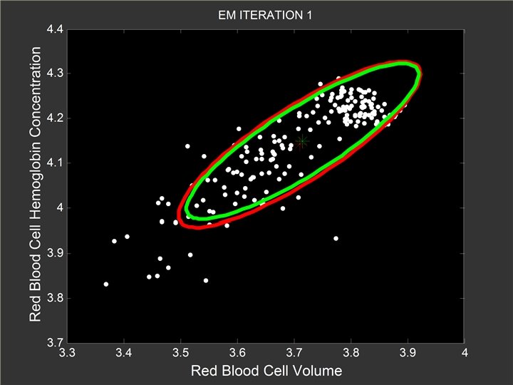
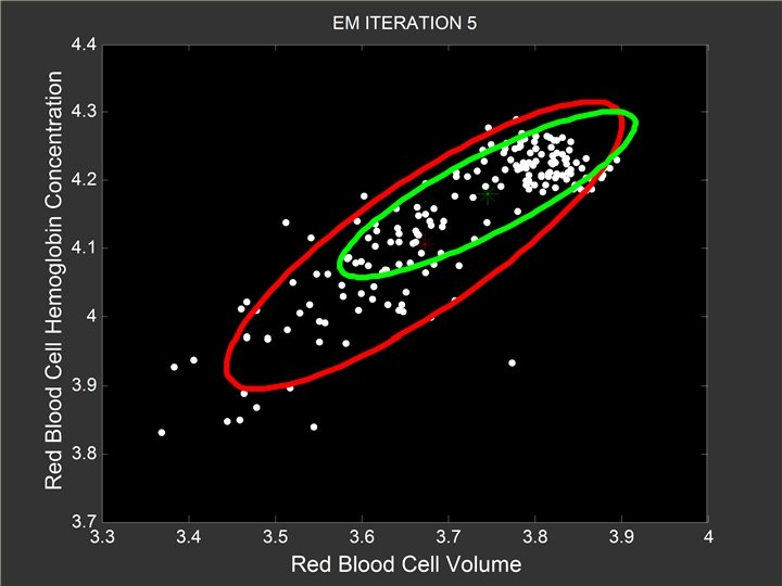
At the 5 -th Iteration l Red Gaussian component slowly shifts toward the left end of the x axis

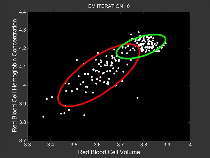
At the 10 -th Iteration l Red Gaussian component still slowly shifts toward the left end of the x axis

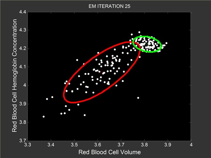
At the 20 -th Iteration l Red Gaussian component make more noticeable shift toward the left end of the x axis

At the 50 -th Iteration l Red Gaussian component is close to the desirable location

At the 100 -th Iteration l The results are almost identical to the ones for the 50 -th iteration

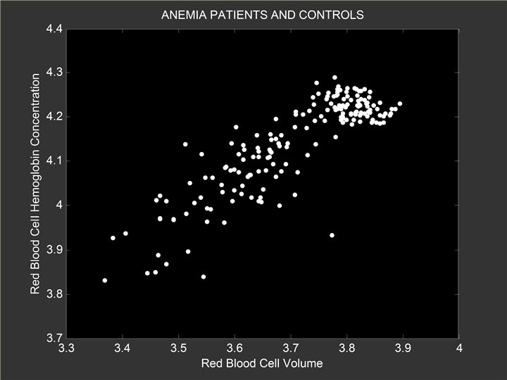
Control Group Anemia Group

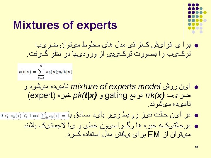
Mixtures of experts μ Ellipsoidal Gating function g 1 Gating Network x g 2 μ 1 Expert Network x g 3 μ 2 Expert Network x μ 3 Expert Network x 67

Hierarchical mixture of experts Linear Gating function 69