Artificial Intelligence Rehearsal Lesson 1 Ram Meshulam 2004

Artificial Intelligence Rehearsal Lesson 1 Ram Meshulam 2004

Solving Problems with Search Algorithms • Input: a problem P. • Preprocessing: – Define states and a state space – Define Operators – Define a start state and goal set of states. • Processing: – Activate a Search algorithm to find a path form start to one of the goal states. 2 Ram Meshulam 2004

Uninformed Search • Uninformed search methods use only information available in the problem definition. – Breadth First Search (BFS) – Depth First Search (DFS) – Iterative DFS (IDA) – Bi-directional search – Uniform Cost Search (a. k. a. Dijkstra alg. ) 3 Ram Meshulam 2004

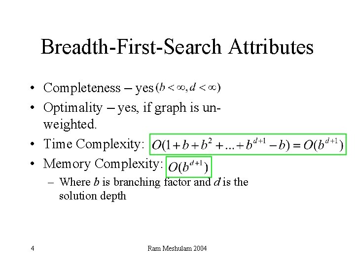
Breadth-First-Search Attributes • Completeness – yes • Optimality – yes, if graph is unweighted. • Time Complexity: • Memory Complexity: – Where b is branching factor and d is the solution depth 4 Ram Meshulam 2004

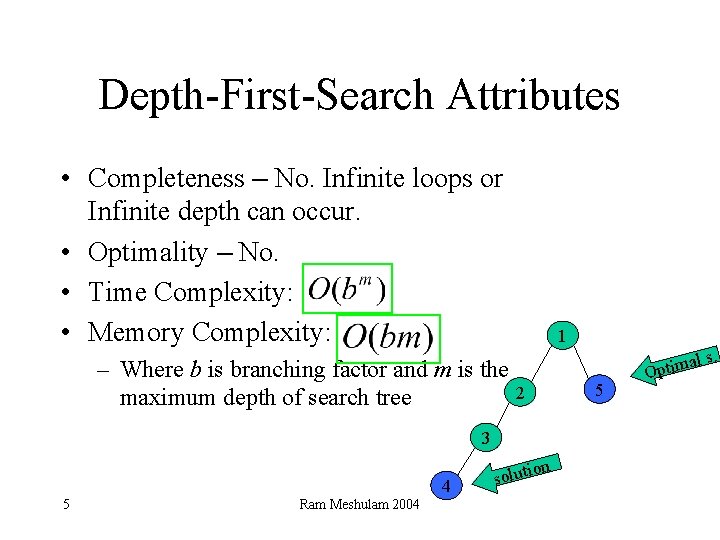
Depth-First-Search Attributes • Completeness – No. Infinite loops or Infinite depth can occur. • Optimality – No. • Time Complexity: • Memory Complexity: – Where b is branching factor and m is the 2 maximum depth of search tree 3 4 5 Ram Meshulam 2004 on soluti 1 5 al Optim s.

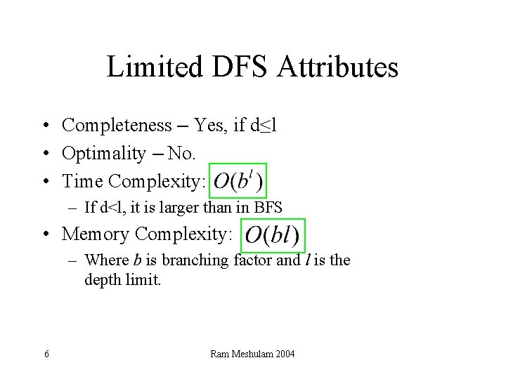
Limited DFS Attributes • Completeness – Yes, if d≤l • Optimality – No. • Time Complexity: – If d<l, it is larger than in BFS • Memory Complexity: – Where b is branching factor and l is the depth limit. 6 Ram Meshulam 2004

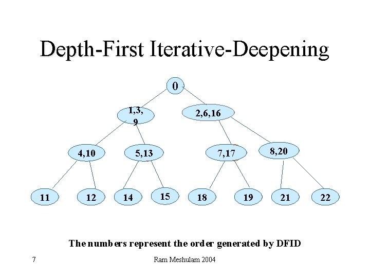
Depth-First Iterative-Deepening 0 1, 3, 9 12 14 8, 20 7, 17 c 5, 13 c 4, 10 11 2, 6, 16 15 c 18 19 21 The numbers represent the order generated by DFID 7 Ram Meshulam 2004 22

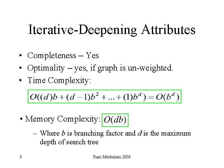
Iterative-Deepening Attributes • Completeness – Yes • Optimality – yes, if graph is un-weighted. • Time Complexity: • Memory Complexity: – Where b is branching factor and d is the maximum depth of search tree 8 Ram Meshulam 2004

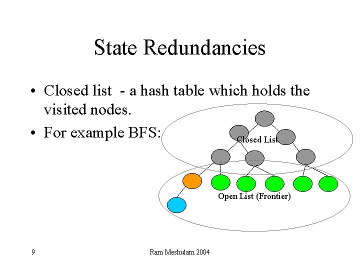
State Redundancies • Closed list - a hash table which holds the visited nodes. • For example BFS: Closed List Open List (Frontier) 9 Ram Meshulam 2004

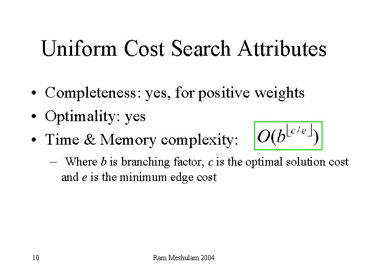
Uniform Cost Search Attributes • Completeness: yes, for positive weights • Optimality: yes • Time & Memory complexity: – Where b is branching factor, c is the optimal solution cost and e is the minimum edge cost 10 Ram Meshulam 2004

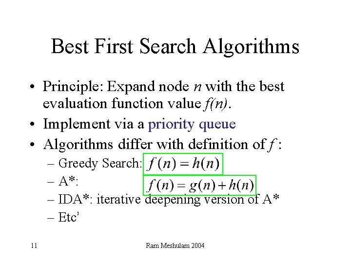
Best First Search Algorithms • Principle: Expand node n with the best evaluation function value f(n). • Implement via a priority queue • Algorithms differ with definition of f : – Greedy Search: – A*: – IDA*: iterative deepening version of A* – Etc’ 11 Ram Meshulam 2004

Best-FS Algorithm Pseudo code 1. Start with open = [initial-state]. 2. While open is not empty do 1. Pick the best node on open. 2. If it is the goal node then return with success. Otherwise find its successors. 3. Assign the successor nodes a score using the evaluation function and add the scored nodes to open 12 Ram Meshulam 2004

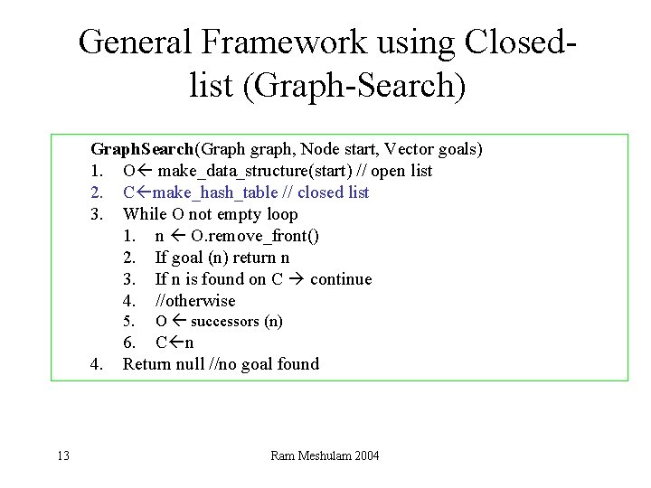
General Framework using Closedlist (Graph-Search) Graph. Search(Graph graph, Node start, Vector goals) 1. O make_data_structure(start) // open list 2. C make_hash_table // closed list 3. While O not empty loop 1. n O. remove_front() 2. If goal (n) return n 3. If n is found on C continue 4. //otherwise 5. 4. 13 O successors (n) 6. C n Return null //no goal found Ram Meshulam 2004

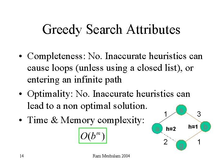
Greedy Search Attributes • Completeness: No. Inaccurate heuristics can cause loops (unless using a closed list), or entering an infinite path • Optimality: No. Inaccurate heuristics can lead to a non optimal solution. s 1 3 • Time & Memory complexity: a 2 14 Ram Meshulam 2004 h=1 h=2 g 1 b

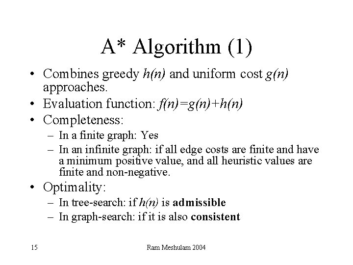
A* Algorithm (1) • Combines greedy h(n) and uniform cost g(n) approaches. • Evaluation function: f(n)=g(n)+h(n) • Completeness: – In a finite graph: Yes – In an infinite graph: if all edge costs are finite and have a minimum positive value, and all heuristic values are finite and non-negative. • Optimality: – In tree-search: if h(n) is admissible – In graph-search: if it is also consistent 15 Ram Meshulam 2004

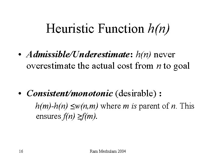
Heuristic Function h(n) • Admissible/Underestimate: h(n) never overestimate the actual cost from n to goal • Consistent/monotonic (desirable) : h(m)-h(n) ≤w(n, m) where m is parent of n. This ensures f(n) ≥f(m). 16 Ram Meshulam 2004

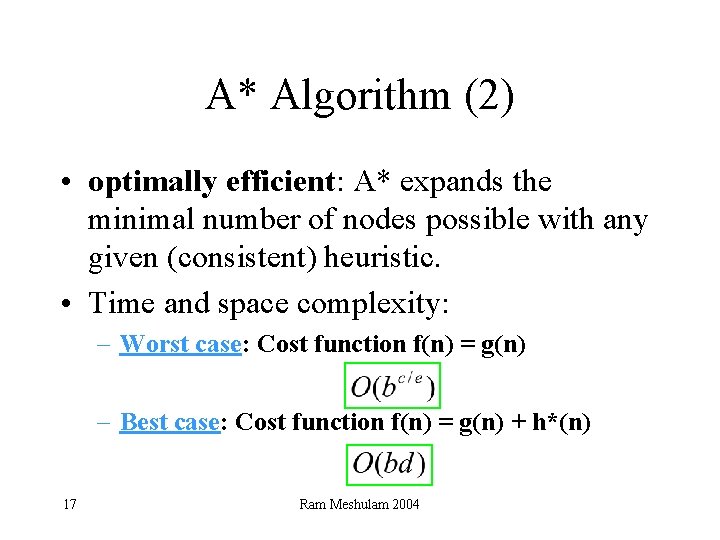
A* Algorithm (2) • optimally efficient: A* expands the minimal number of nodes possible with any given (consistent) heuristic. • Time and space complexity: – Worst case: Cost function f(n) = g(n) – Best case: Cost function f(n) = g(n) + h*(n) 17 Ram Meshulam 2004

Duplicate Pruning • Do not enter the father of the current state – With or without using closed-list • Using a closed-list, check the closed list before entering new nodes to the open list – Note: in A*, h has to be consistent! – Do not remove the original check • Using a stack, check the current branch and stack status before entering new nodes 18 Ram Meshulam 2004

IDA* Algorithm • Each iteration is a depth-first search that keeps track of the cost evaluation f = g + h of each node generated. • The cost threshold is initialized to the heuristic of the initial state. • If a node is generated whose cost exceeds the threshold for that iteration, its path is cut off. 19 Ram Meshulam 2004

IDA* Attributes • The cost threshold increases in each iteration to the total cost of the lowest-cost node that was pruned during the previous iteration. • The algorithm terminates when a goal state is reached whose total cost does not exceed the current threshold. • Completeness and Optimality: Like A* • Space complexity: • Time complexity*: 20 Ram Meshulam 2004

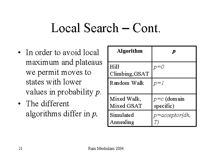
Local Search – Cont. • In order to avoid local maximum and plateaus we permit moves to states with lower values in probability p. • The different algorithms differ in p. 21 Algorithm p Hill p=0 Climbing, GSAT Random Walk p=1 Mixed Walk, Mixed GSAT p=c (domain specific) Simulated Annealing p=acceptor(dh, T) Ram Meshulam 2004

Hill Climbing • Always choose the next best successor • Stop when no improvement possible • In order to avoid plateaus and local maximum: - Sideways move - Stochastic hill climbing - Random-restart algorithm 22 Ram Meshulam 2004

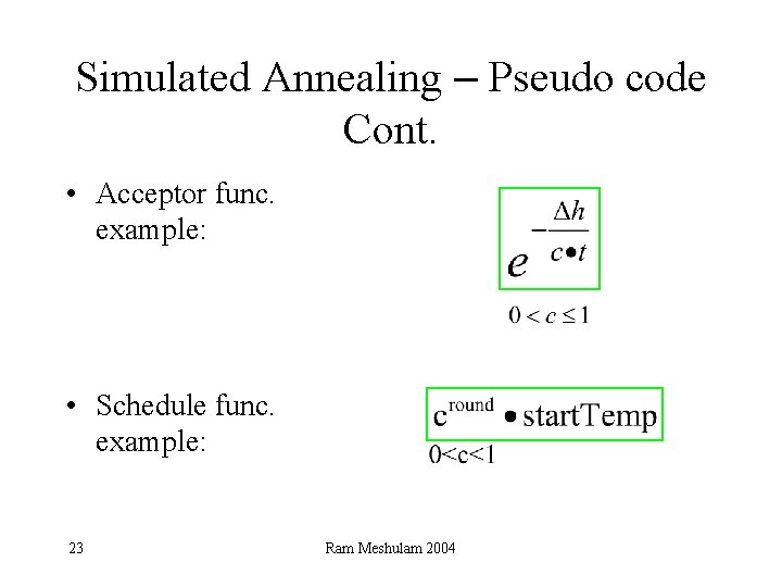
Simulated Annealing – Pseudo code Cont. • Acceptor func. example: • Schedule func. example: 23 Ram Meshulam 2004

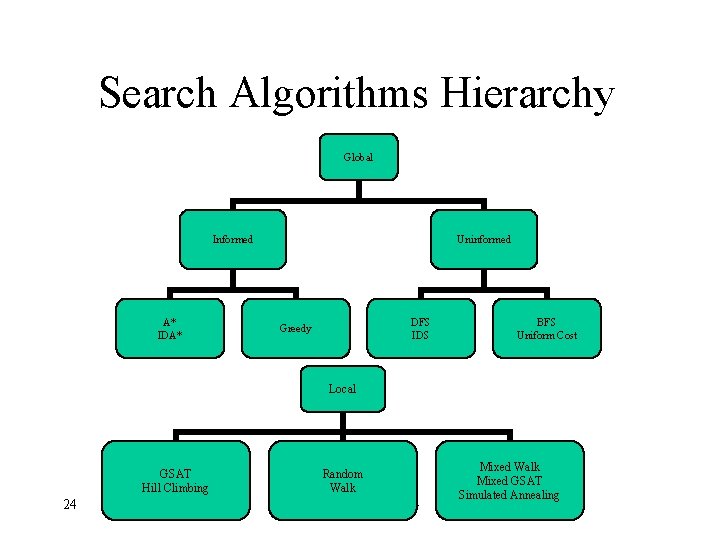
Search Algorithms Hierarchy Global Informed A* IDA* Uninformed DFS IDS Greedy BFS Uniform Cost Local GSAT Hill Climbing 24 Random Walk Ram Meshulam 2004 Mixed Walk Mixed GSAT Simulated Annealing

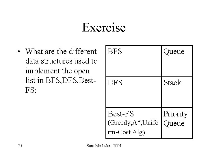
Exercise • What are the different data structures used to implement the open list in BFS, DFS, Best. FS: BFS Queue DFS Stack Best-FS Priority (Greedy, A*, Unifo Queue rm-Cost Alg). 25 Ram Meshulam 2004

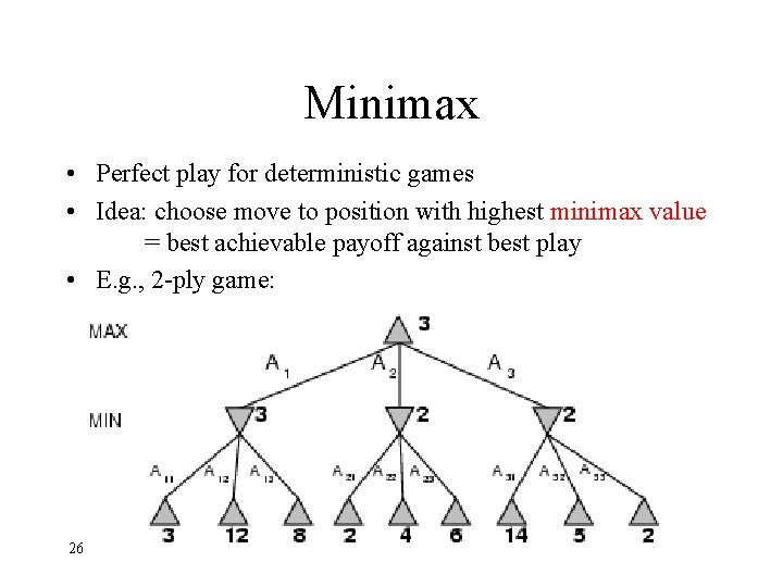
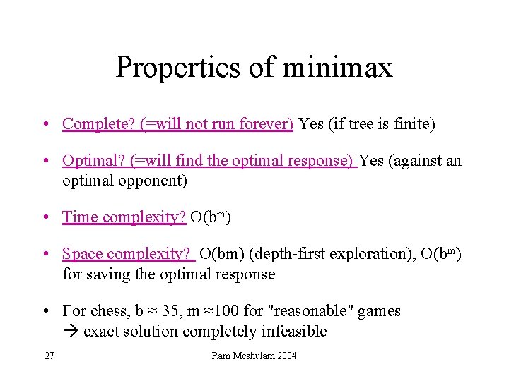
Minimax • Perfect play for deterministic games • Idea: choose move to position with highest minimax value = best achievable payoff against best play • E. g. , 2 -ply game: 26 Ram Meshulam 2004

Properties of minimax • Complete? (=will not run forever) Yes (if tree is finite) • Optimal? (=will find the optimal response) Yes (against an optimal opponent) • Time complexity? O(bm) • Space complexity? O(bm) (depth-first exploration), O(bm) for saving the optimal response • For chess, b ≈ 35, m ≈100 for "reasonable" games exact solution completely infeasible 27 Ram Meshulam 2004

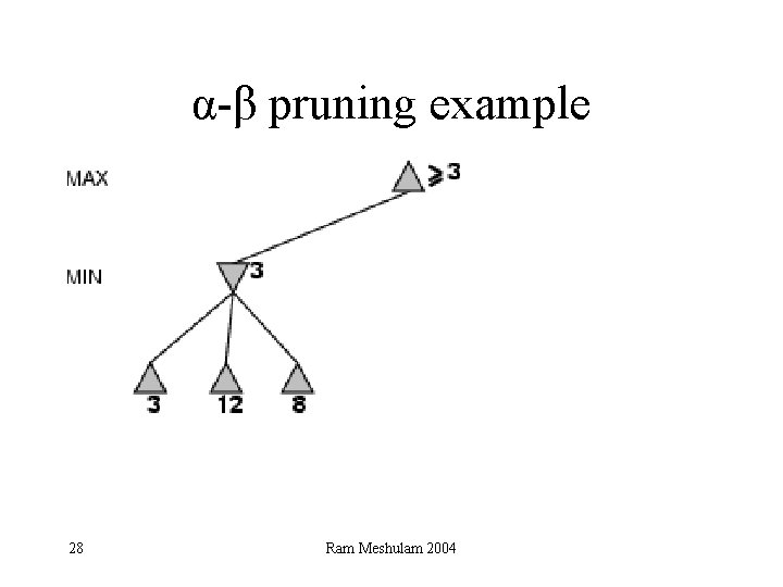
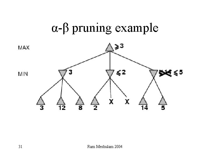
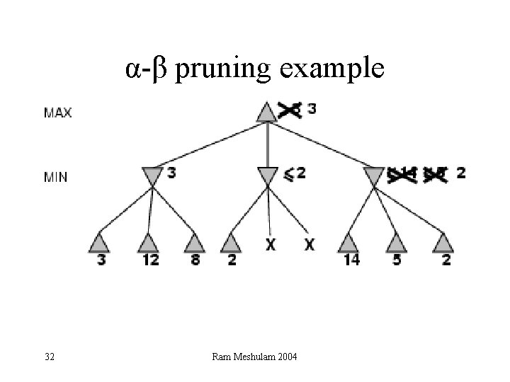
α-β pruning example 28 Ram Meshulam 2004

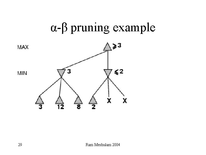
α-β pruning example 29 Ram Meshulam 2004

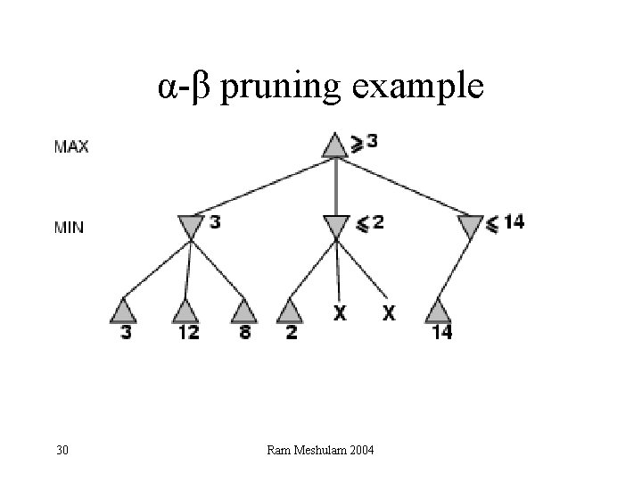
α-β pruning example 30 Ram Meshulam 2004

α-β pruning example 31 Ram Meshulam 2004

α-β pruning example 32 Ram Meshulam 2004

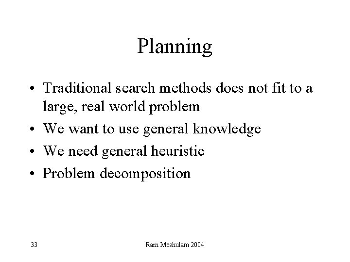
Planning • Traditional search methods does not fit to a large, real world problem • We want to use general knowledge • We need general heuristic • Problem decomposition 33 Ram Meshulam 2004

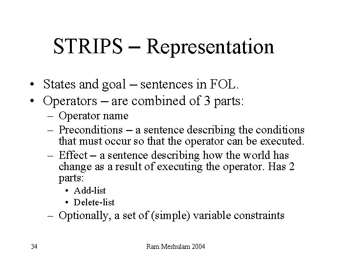
STRIPS – Representation • States and goal – sentences in FOL. • Operators – are combined of 3 parts: – Operator name – Preconditions – a sentence describing the conditions that must occur so that the operator can be executed. – Effect – a sentence describing how the world has change as a result of executing the operator. Has 2 parts: • Add-list • Delete-list – Optionally, a set of (simple) variable constraints 34 Ram Meshulam 2004

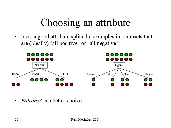
Choosing an attribute • Idea: a good attribute splits the examples into subsets that are (ideally) "all positive" or "all negative" • Patrons? is a better choice 35 Ram Meshulam 2004

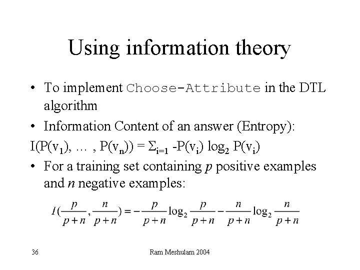
Using information theory • To implement Choose-Attribute in the DTL algorithm • Information Content of an answer (Entropy): I(P(v 1), … , P(vn)) = Σi=1 -P(vi) log 2 P(vi) • For a training set containing p positive examples and n negative examples: 36 Ram Meshulam 2004

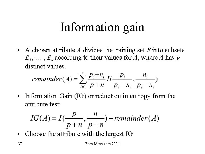
Information gain • A chosen attribute A divides the training set E into subsets E 1, … , Ev according to their values for A, where A has v distinct values. • Information Gain (IG) or reduction in entropy from the attribute test: • Choose the attribute with the largest IG 37 Ram Meshulam 2004

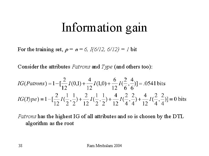
Information gain For the training set, p = n = 6, I(6/12, 6/12) = 1 bit Consider the attributes Patrons and Type (and others too): Patrons has the highest IG of all attributes and so is chosen by the DTL algorithm as the root 38 Ram Meshulam 2004

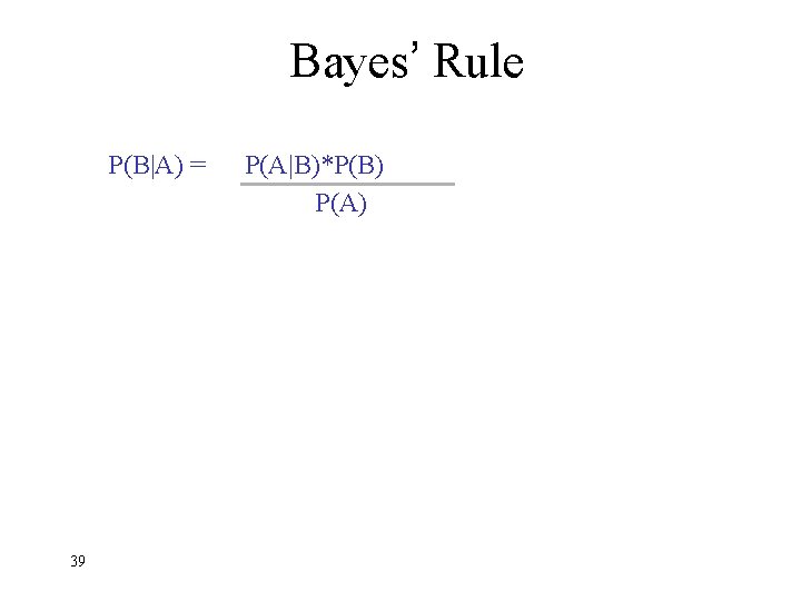
Bayes’ Rule P(B|A) = 39 P(A|B)*P(B) P(A)

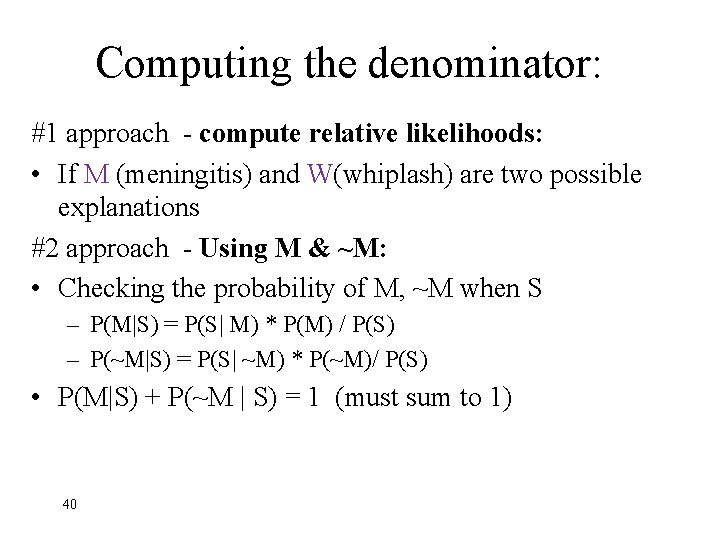
Computing the denominator: #1 approach - compute relative likelihoods: • If M (meningitis) and W(whiplash) are two possible explanations #2 approach - Using M & ~M: • Checking the probability of M, ~M when S – P(M|S) = P(S| M) * P(M) / P(S) – P(~M|S) = P(S| ~M) * P(~M)/ P(S) • P(M|S) + P(~M | S) = 1 (must sum to 1) 40

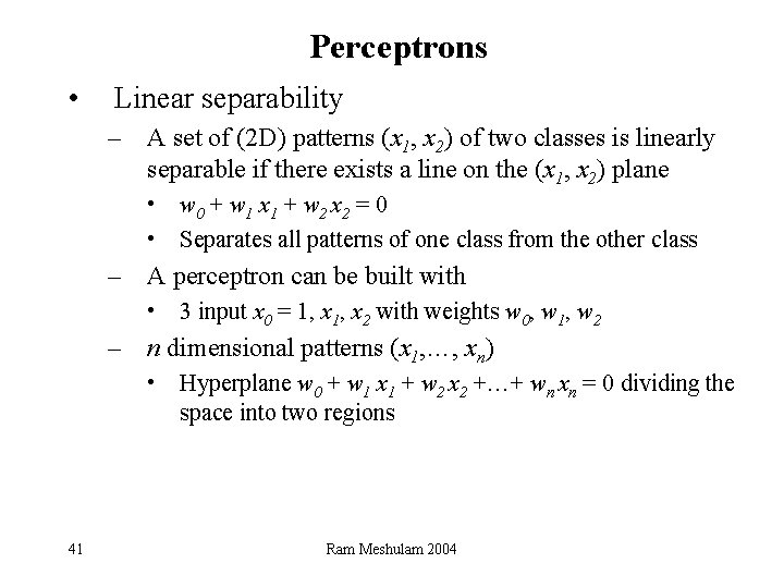
Perceptrons • Linear separability – A set of (2 D) patterns (x 1, x 2) of two classes is linearly separable if there exists a line on the (x 1, x 2) plane • w 0 + w 1 x 1 + w 2 x 2 = 0 • Separates all patterns of one class from the other class – A perceptron can be built with • 3 input x 0 = 1, x 2 with weights w 0, w 1, w 2 – n dimensional patterns (x 1, …, xn) • Hyperplane w 0 + w 1 x 1 + w 2 x 2 +…+ wn xn = 0 dividing the space into two regions 41 Ram Meshulam 2004

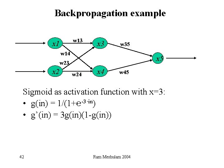
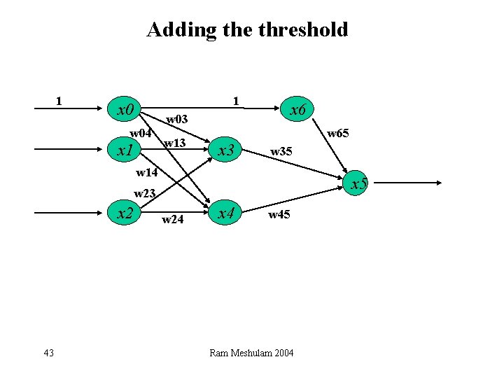
Backpropagation example w 13 x 1 x 3 w 35 w 14 x 5 w 23 x 2 w 24 x 4 w 45 Sigmoid as activation function with x=3: • g(in) = 1/(1+℮-3·in) • g’(in) = 3 g(in)(1 -g(in)) 42 Ram Meshulam 2004

Adding the threshold 1 1 x 0 x 6 w 03 w 04 x 1 w 13 w 65 x 3 w 35 w 14 x 5 w 23 x 2 43 w 24 x 4 w 45 Ram Meshulam 2004

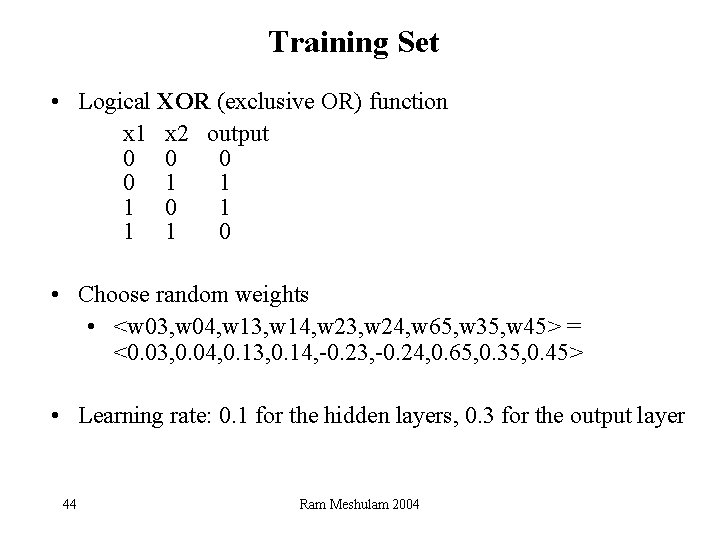
Training Set • Logical XOR (exclusive OR) function x 1 x 2 output 0 0 1 1 1 0 • Choose random weights • <w 03, w 04, w 13, w 14, w 23, w 24, w 65, w 35, w 45> = <0. 03, 0. 04, 0. 13, 0. 14, -0. 23, -0. 24, 0. 65, 0. 35, 0. 45> • Learning rate: 0. 1 for the hidden layers, 0. 3 for the output layer 44 Ram Meshulam 2004

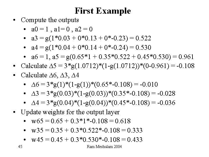
First Example • Compute the outputs • a 0 = 1 , a 1= 0 , a 2 = 0 • a 3 = g(1*0. 03 + 0*0. 13 + 0*-0. 23) = 0. 522 • a 4 = g(1*0. 04 + 0*0. 14 + 0*-0. 24) = 0. 530 • a 6 = 1, a 5 = g(0. 65*1 + 0. 35*0. 522 + 0. 45*0. 530) = 0. 961 • Calculate ∆5 = 3*g(1. 0712)*(1 -g(1. 0712))*(0 -0. 961) = -0. 108 • Calculate ∆6, ∆3, ∆4 • ∆6 = 3*g(1)*(1 -g(1))*(0. 65*-0. 108) = -0. 010 • ∆3 = 3*g(0. 03)*(1 -g(0. 03))*(0. 35*-0. 108) = -0. 028 • ∆4 = 3*g(0. 04)*(1 -g(0. 04))*(0. 45*-0. 108) = -0. 036 • Update weights for the output layer • w 65 = 0. 65 + 0. 3*1*-0. 108 = 0. 618 • w 35 = 0. 35 + 0. 3*0. 522*-0. 108 = 0. 333 • w 45 = 0. 45 + 0. 3*0. 530*-0. 108 = 0. 433 45 Ram Meshulam 2004

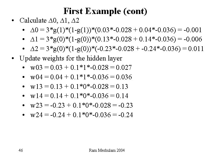
First Example (cont) • Calculate ∆0, ∆1, ∆2 • ∆0 = 3*g(1)*(1 -g(1))*(0. 03*-0. 028 + 0. 04*-0. 036) = -0. 001 • ∆1 = 3*g(0)*(1 -g(0))*(0. 13*-0. 028 + 0. 14*-0. 036) = -0. 006 • ∆2 = 3*g(0)*(1 -g(0))*(-0. 23*-0. 028 + -0. 24*-0. 036) = 0. 011 • Update weights for the hidden layer • w 03 = 0. 03 + 0. 1*1*-0. 028 = 0. 027 • w 04 = 0. 04 + 0. 1*1*-0. 036 = 0. 036 • w 13 = 0. 13 + 0. 1*0*-0. 028 = 0. 13 • w 14 = 0. 14 + 0. 1*0*-0. 036 = 0. 14 • w 23 = -0. 23 + 0. 1*0*-0. 028 = -0. 23 • w 24 = -0. 24 + 0. 1*0*-0. 036 = -0. 24 46 Ram Meshulam 2004

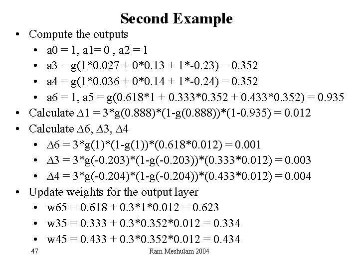
Second Example • Compute the outputs • a 0 = 1, a 1= 0 , a 2 = 1 • a 3 = g(1*0. 027 + 0*0. 13 + 1*-0. 23) = 0. 352 • a 4 = g(1*0. 036 + 0*0. 14 + 1*-0. 24) = 0. 352 • a 6 = 1, a 5 = g(0. 618*1 + 0. 333*0. 352 + 0. 433*0. 352) = 0. 935 • Calculate ∆1 = 3*g(0. 888)*(1 -g(0. 888))*(1 -0. 935) = 0. 012 • Calculate ∆6, ∆3, ∆4 • ∆6 = 3*g(1)*(1 -g(1))*(0. 618*0. 012) = 0. 001 • ∆3 = 3*g(-0. 203)*(1 -g(-0. 203))*(0. 333*0. 012) = 0. 003 • ∆4 = 3*g(-0. 204)*(1 -g(-0. 204))*(0. 433*0. 012) = 0. 004 • Update weights for the output layer • w 65 = 0. 618 + 0. 3*1*0. 012 = 0. 623 • w 35 = 0. 333 + 0. 3*0. 352*0. 012 = 0. 334 • w 45 = 0. 433 + 0. 3*0. 352*0. 012 = 0. 434 47 Ram Meshulam 2004

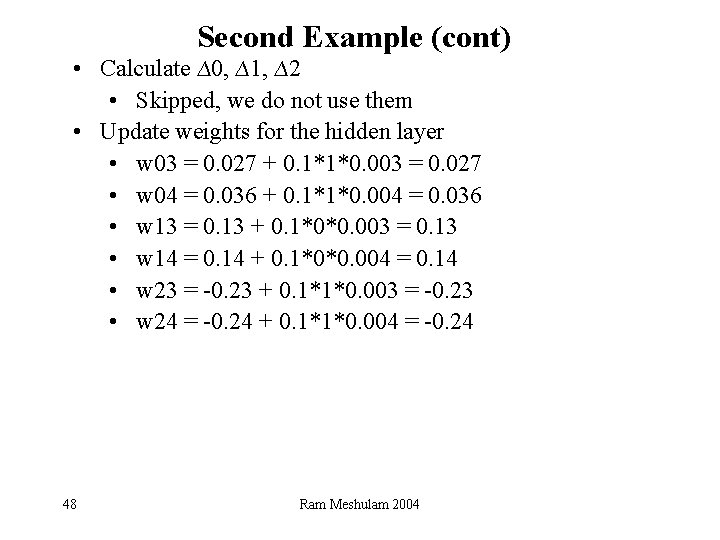
Second Example (cont) • Calculate ∆0, ∆1, ∆2 • Skipped, we do not use them • Update weights for the hidden layer • w 03 = 0. 027 + 0. 1*1*0. 003 = 0. 027 • w 04 = 0. 036 + 0. 1*1*0. 004 = 0. 036 • w 13 = 0. 13 + 0. 1*0*0. 003 = 0. 13 • w 14 = 0. 14 + 0. 1*0*0. 004 = 0. 14 • w 23 = -0. 23 + 0. 1*1*0. 003 = -0. 23 • w 24 = -0. 24 + 0. 1*1*0. 004 = -0. 24 48 Ram Meshulam 2004

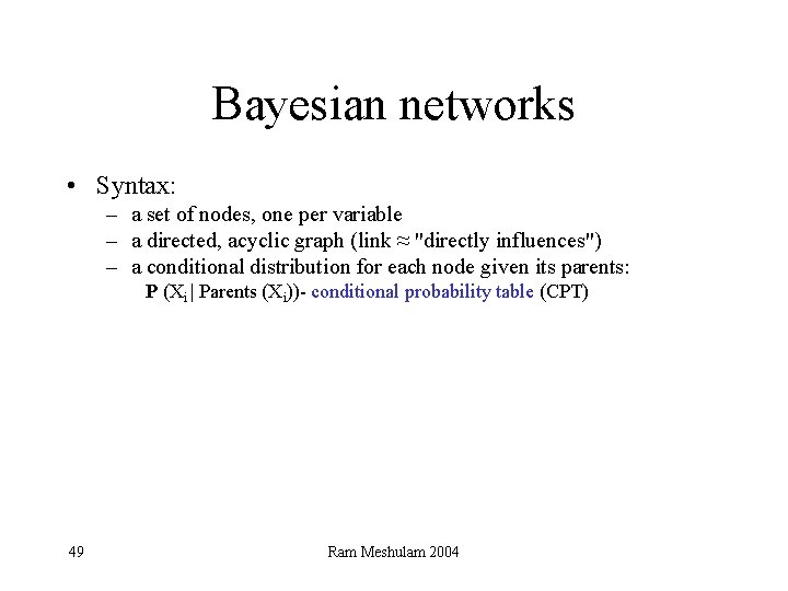
Bayesian networks • Syntax: – a set of nodes, one per variable – a directed, acyclic graph (link ≈ "directly influences") – a conditional distribution for each node given its parents: P (Xi | Parents (Xi))- conditional probability table (CPT) 49 Ram Meshulam 2004

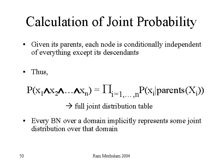
Calculation of Joint Probability • Given its parents, each node is conditionally independent of everything except its descendants • Thus, P(x 1 x 2 … xn) = Pi=1, …, n. P(xi|parents(Xi)) full joint distribution table • Every BN over a domain implicitly represents some joint distribution over that domain 50 Ram Meshulam 2004

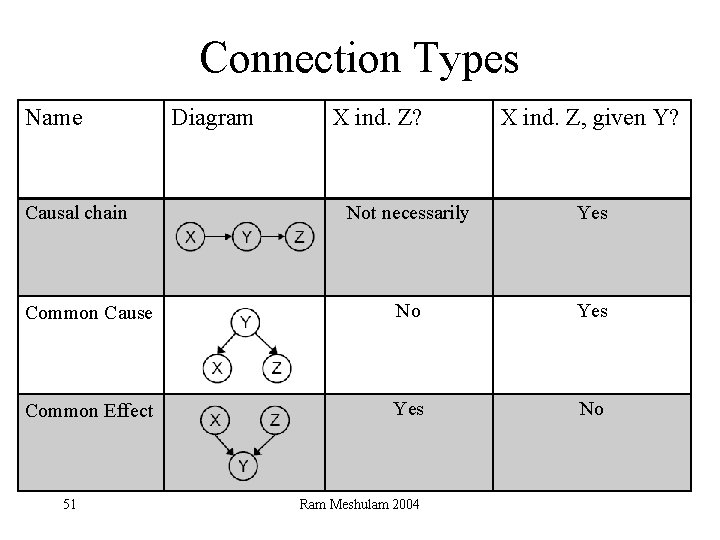
Connection Types Name Causal chain Diagram X ind. Z? X ind. Z, given Y? Not necessarily Yes Common Cause No Yes Common Effect Yes No 51 Ram Meshulam 2004

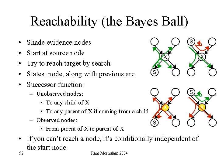
Reachability (the Bayes Ball) • • • Shade evidence nodes Start at source node Try to reach target by search States: node, along with previous arc Successor function: – Unobserved nodes: • To any child of X • To any parent of X if coming from a child – Observed nodes: • From parent of X to parent of X • If you can’t reach a node, it’s conditionally independent of the start node 52 Ram Meshulam 2004

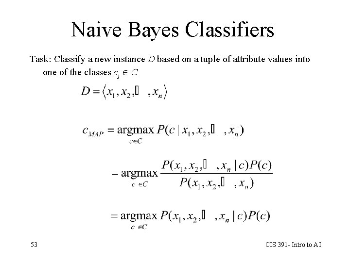
Naive Bayes Classifiers Task: Classify a new instance D based on a tuple of attribute values into one of the classes cj C 53 CIS 391 - Intro to AI

Robots Environment Assumptions • Static - to be able to guarantee completeness • Inaccessible - greater impact on the on-line version • Non-deterministic (move 5 M, but able to move 5. 1 M) • Continuous – Exact cellular decomposition – Approximate cellular decomposition 54

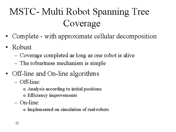
MSTC- Multi Robot Spanning Tree Coverage • Complete - with approximate cellular decomposition • Robust – Coverage completed as long as one robot is alive – The robustness mechanism is simple • Off-line and On-line algorithms – Off-line: o Analysis according to initial positions o Efficiency improvements – On-line: o Implemented on simulation of real-robots 55

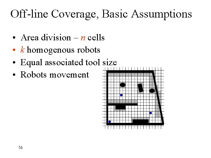
Off-line Coverage, Basic Assumptions • • Area division – n cells k homogenous robots Equal associated tool size Robots movement 56

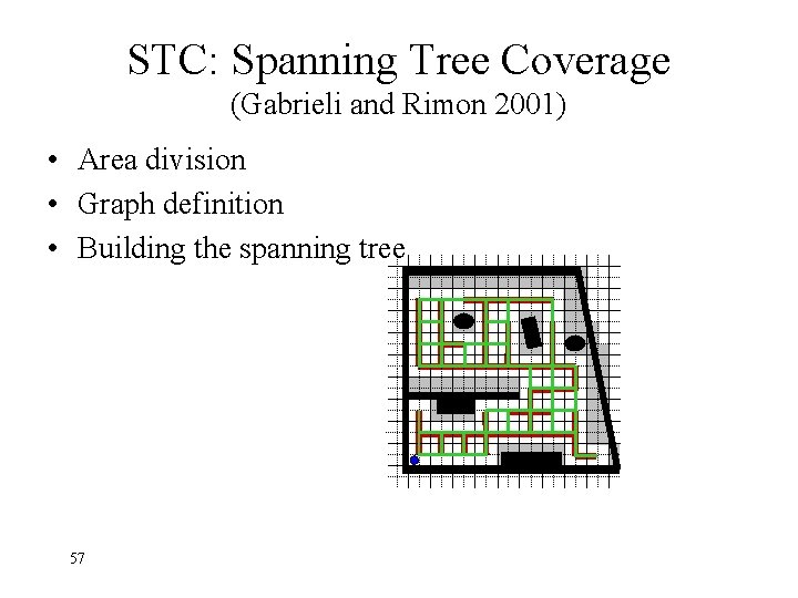
STC: Spanning Tree Coverage (Gabrieli and Rimon 2001) • Area division • Graph definition • Building the spanning tree 57

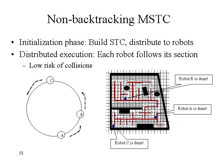
Non-backtracking MSTC • Initialization phase: Build STC, distribute to robots • Distributed execution: Each robot follows its section – Low risk of collisions Robot B is done! C Robot A is done! B A Robot C is done! 58

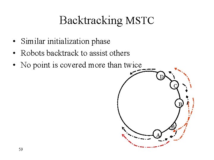
Backtracking MSTC • Similar initialization phase • Robots backtrack to assist others • No point is covered more than twice D C B B A 59