Artificial Intelligence 12 Two Layer ANNs Course V

Artificial Intelligence 12. Two Layer ANNs Course V 231 Department of Computing Imperial College, London © Simon Colton

Non Symbolic Representations l Decision trees can be easily read – – l Non-symbolic representations – l A disjunction of conjunctions (logic) We call this a symbolic representation More numerical in nature, more difficult to read Artificial Neural Networks (ANNs) – – A Non-symbolic representation scheme They embed a giant mathematical function l – To take inputs and compute an output which is interpreted as a categorisation Often shortened to “Neural Networks” l Don’t confuse them with real neural networks (in heads)

Function Learning l Map categorisation learning to numerical problem – – l Each category given a number Or a range of real valued numbers (e. g. , 0. 5 - 0. 9) Function learning examples – – – Input = 1, 2, 3, 4 Output = 1, 4, 9, 16 Here the concept to learn is squaring integers Input = [1, 2, 3], [2, 3, 4], [3, 4, 5], [4, 5, 6] Output = 1, 5, 11, 19 Here the concept is: [a, b, c] -> a*c - b l l The calculation is more complicated than in the first example Neural networks: – – Calculation is much more complicated in general But it is still just a numerical calculation

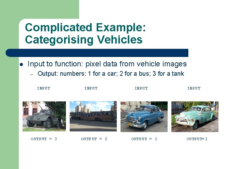
Complicated Example: Categorising Vehicles l Input to function: pixel data from vehicle images – Output: numbers: 1 for a car; 2 for a bus; 3 for a tank INPUT OUTPUT = 3 INPUT OUTPUT = 2 INPUT OUTPUT = 1 INPUT OUTPUT=1

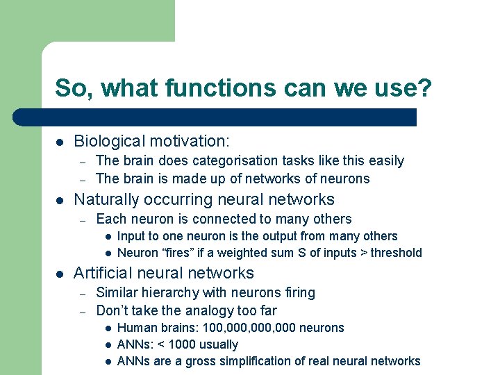
So, what functions can we use? l Biological motivation: – – l The brain does categorisation tasks like this easily The brain is made up of networks of neurons Naturally occurring neural networks – Each neuron is connected to many others l l l Input to one neuron is the output from many others Neuron “fires” if a weighted sum S of inputs > threshold Artificial neural networks – – Similar hierarchy with neurons firing Don’t take the analogy too far l l l Human brains: 100, 000, 000 neurons ANNs: < 1000 usually ANNs are a gross simplification of real neural networks

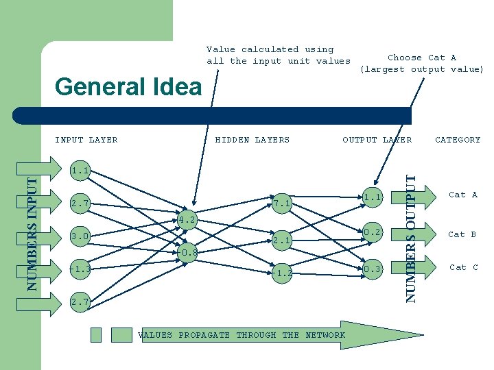
Value calculated using all the input unit values General Idea HIDDEN LAYERS OUTPUT LAYER NUMBERS INPUT 1. 1 2. 7 7. 1 1. 1 4. 2 3. 0 2. 1 0. 2 -0. 8 -1. 3 -1. 2 2. 7 VALUES PROPAGATE THROUGH THE NETWORK 0. 3 NUMBERS OUTPUT INPUT LAYER Choose Cat A (largest output value) CATEGORY Cat A Cat B Cat C

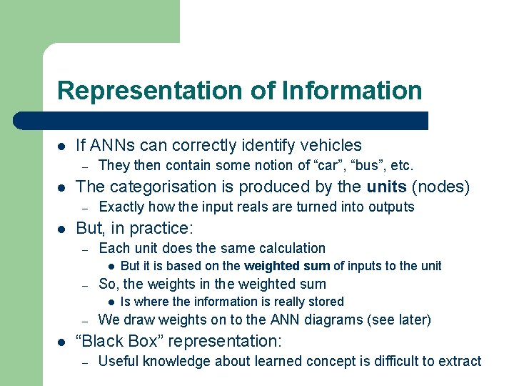
Representation of Information l If ANNs can correctly identify vehicles – l The categorisation is produced by the units (nodes) – l They then contain some notion of “car”, “bus”, etc. Exactly how the input reals are turned into outputs But, in practice: – Each unit does the same calculation l – So, the weights in the weighted sum l – l But it is based on the weighted sum of inputs to the unit Is where the information is really stored We draw weights on to the ANN diagrams (see later) “Black Box” representation: – Useful knowledge about learned concept is difficult to extract

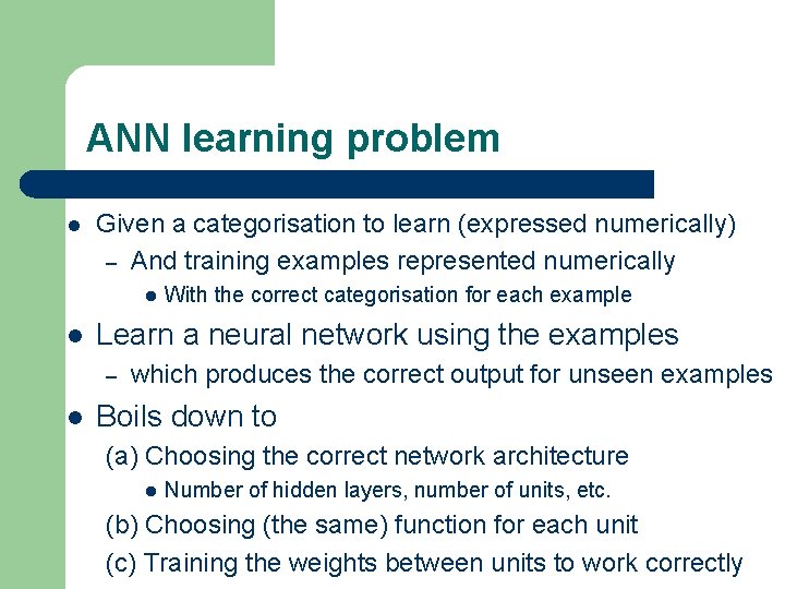
ANN learning problem l Given a categorisation to learn (expressed numerically) – And training examples represented numerically l l Learn a neural network using the examples – l With the correct categorisation for each example which produces the correct output for unseen examples Boils down to (a) Choosing the correct network architecture l Number of hidden layers, number of units, etc. (b) Choosing (the same) function for each unit (c) Training the weights between units to work correctly

Special Cases l Generally, can have many hidden layers – l Next lecture: – – l In practice, usually one or two Look at ANNs with one hidden layer Multi-layer ANNs This lecture: – – – Look at ANNs with no hidden layer Two layer ANNs Perceptrons

Perceptrons l l Multiple input nodes Single output node – – l Useful to study because – l Takes a weighted sum of the inputs, call this S Unit function calculates the output for the network We can use perceptrons to build larger networks Perceptrons have limited representational abilities – We will look at concepts they can’t learn later

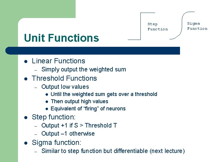
Step Function Unit Functions l Linear Functions – l Simply output the weighted sum Threshold Functions – Output low values l l Step function: – – l Until the weighted sum gets over a threshold Then output high values Equivalent of “firing” of neurons Output +1 if S > Threshold T Output – 1 otherwise Sigma function: – Similar to step function but differentiable (next lecture) Sigma Function

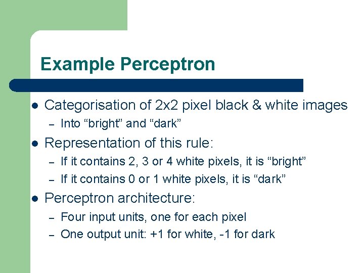
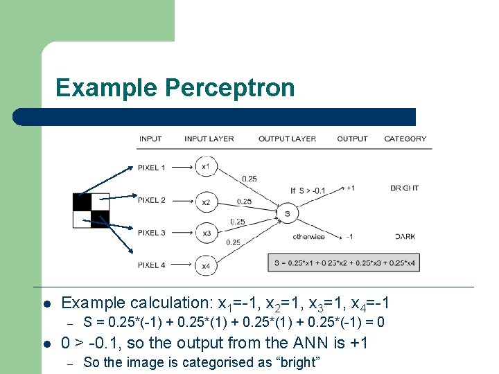
Example Perceptron l Categorisation of 2 x 2 pixel black & white images – l Representation of this rule: – – l Into “bright” and “dark” If it contains 2, 3 or 4 white pixels, it is “bright” If it contains 0 or 1 white pixels, it is “dark” Perceptron architecture: – – Four input units, one for each pixel One output unit: +1 for white, -1 for dark

Example Perceptron l Example calculation: x 1=-1, x 2=1, x 3=1, x 4=-1 – l S = 0. 25*(-1) + 0. 25*(1) + 0. 25*(-1) = 0 0 > -0. 1, so the output from the ANN is +1 – So the image is categorised as “bright”

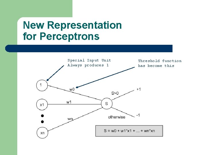
Learning in Perceptrons l Need to learn – – l Make calculations easier by – l Both the weights between input and output units And the value for the threshold Thinking of the threshold as a weight from a special input unit where the output from the unit is always 1 Exactly the same result – But we only have to worry about learning weights

New Representation for Perceptrons Special Input Unit Always produces 1 Threshold function has become this

Learning Algorithm l l Weights are set randomly initially For each training example E – – Calculate the observed output from the ANN, o(E) If the target output t(E) is different to o(E) l l Then tweak all the weights so that o(E) gets closer to t(E) Tweaking is done by perceptron training rule (next slide) This routine is done for every example E Don’t necessarily stop when all examples used – – Repeat the cycle again (an ‘epoch’) Until the ANN produces the correct output l For all the examples in the training set (or good enough)

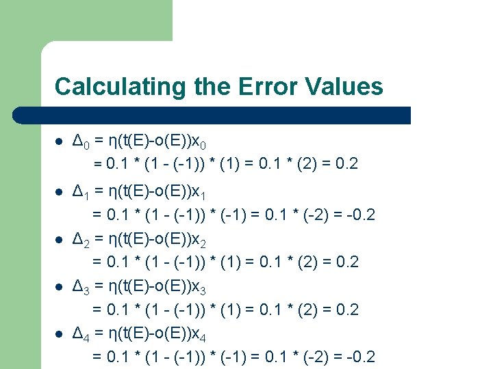
Perceptron Training Rule l When t(E) is different to o(E) – – – l Add on Δi to weight wi Where Δi = η(t(E)-o(E))xi Do this for every weight in the network Interpretation: – – (t(E) – o(E)) will either be +2 or – 2 [cannot be the same sign] So we can think of the addition of Δi as the movement of the weight in a direction l – Which will improve the networks performance with respect to E Multiplication by xi l Moves it more if the input is bigger

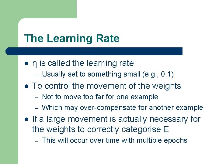
The Learning Rate l η is called the learning rate – l To control the movement of the weights – – l Usually set to something small (e. g. , 0. 1) Not to move too far for one example Which may over-compensate for another example If a large movement is actually necessary for the weights to correctly categorise E – This will occur over time with multiple epochs

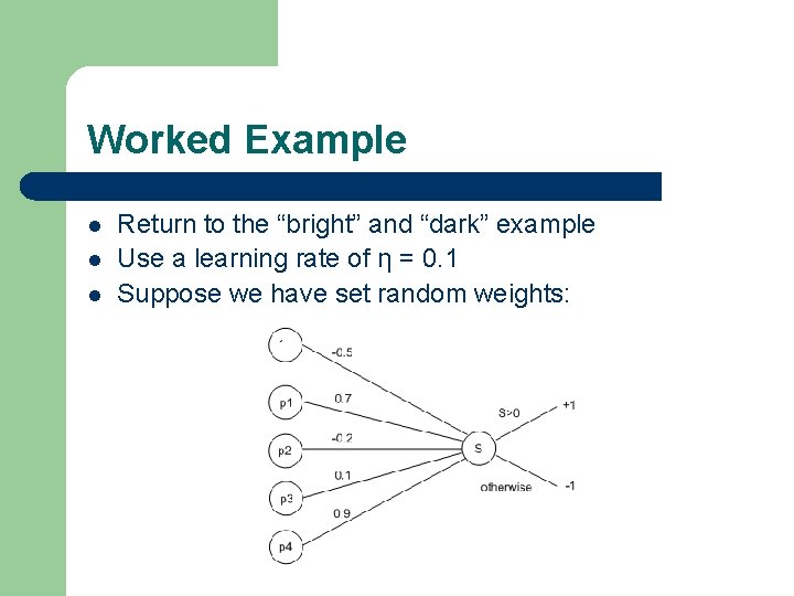
Worked Example l l l Return to the “bright” and “dark” example Use a learning rate of η = 0. 1 Suppose we have set random weights:

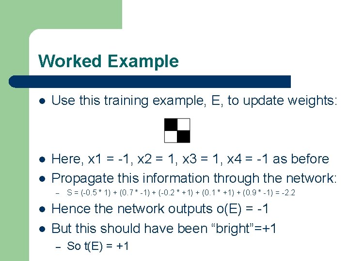
Worked Example l Use this training example, E, to update weights: l Here, x 1 = -1, x 2 = 1, x 3 = 1, x 4 = -1 as before Propagate this information through the network: l – l l S = (-0. 5 * 1) + (0. 7 * -1) + (-0. 2 * +1) + (0. 1 * +1) + (0. 9 * -1) = -2. 2 Hence the network outputs o(E) = -1 But this should have been “bright”=+1 – So t(E) = +1

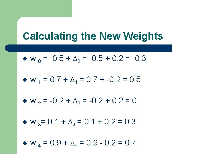
Calculating the New Weights l w’ 0 = -0. 5 + Δ 0 = -0. 5 + 0. 2 = -0. 3 l w’ 1 = 0. 7 + Δ 1 = 0. 7 + -0. 2 = 0. 5 l w’ 2 = -0. 2 + Δ 2 = -0. 2 + 0. 2 = 0 l w’ 3= 0. 1 + Δ 3 = 0. 1 + 0. 2 = 0. 3 l w’ 4 = 0. 9 + Δ 4 = 0. 9 - 0. 2 = 0. 7

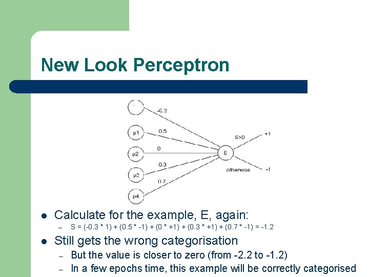
New Look Perceptron l Calculate for the example, E, again: – l S = (-0. 3 * 1) + (0. 5 * -1) + (0 * +1) + (0. 3 * +1) + (0. 7 * -1) = -1. 2 Still gets the wrong categorisation – – But the value is closer to zero (from -2. 2 to -1. 2) In a few epochs time, this example will be correctly categorised

Learning Abilities of Perceptrons l l Perceptrons are a very simple network Computational learning theory – Study of which concepts can and can’t be learned l l By particular learning techniques (representation, method) Minsky and Papert’s influencial book – – – Showed the limitations of perceptrons Cannot learn some simple boolean functions Caused a “winter” of research for ANNs in AI l l l People thought it represented a fundamental limitation But perceptrons are the simplest network ANNS were revived by neuroscientists, etc.

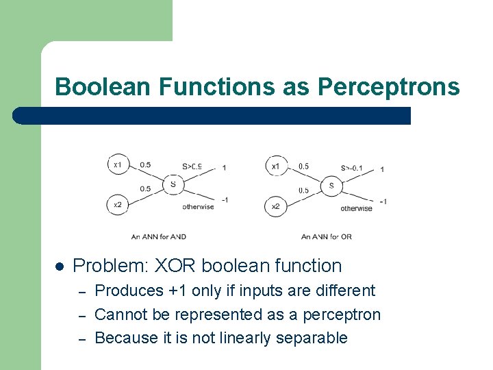
Boolean Functions l l Take in two inputs (-1 or +1) Produce one output (-1 or +1) In other contexts, use 0 and 1 Example: AND function – l Example: OR function – l Produces +1 only if both inputs are +1 Produces +1 if either inputs are +1 Related to the logical connectives from F. O. L.

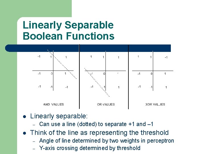
Boolean Functions as Perceptrons l Problem: XOR boolean function – – – Produces +1 only if inputs are different Cannot be represented as a perceptron Because it is not linearly separable

Linearly Separable Boolean Functions l Linearly separable: – l Can use a line (dotted) to separate +1 and – 1 Think of the line as representing the threshold – – Angle of line determined by two weights in perceptron Y-axis crossing determined by threshold

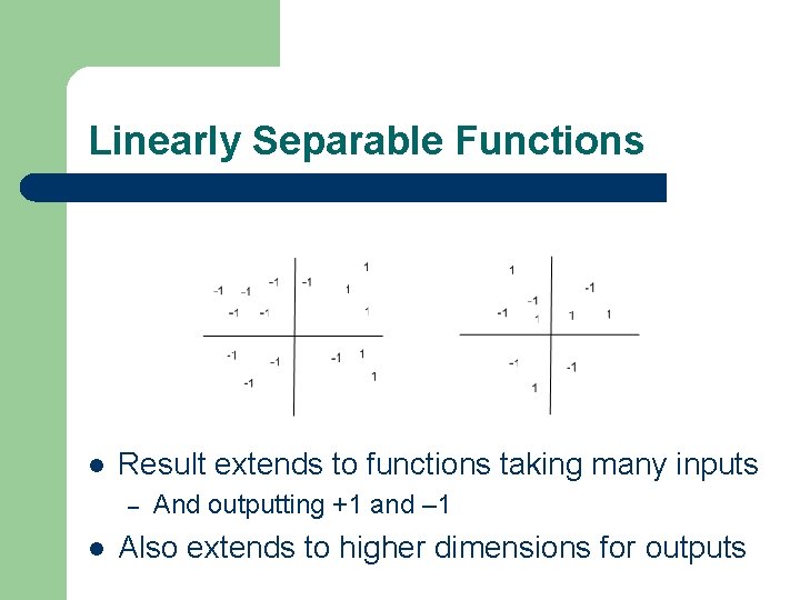
Linearly Separable Functions l Result extends to functions taking many inputs – l And outputting +1 and – 1 Also extends to higher dimensions for outputs