Artificial Intelligence 13 MultiLayer ANNs Course V 231

Artificial Intelligence 13. Multi-Layer ANNs Course V 231 Department of Computing Imperial College © Simon Colton

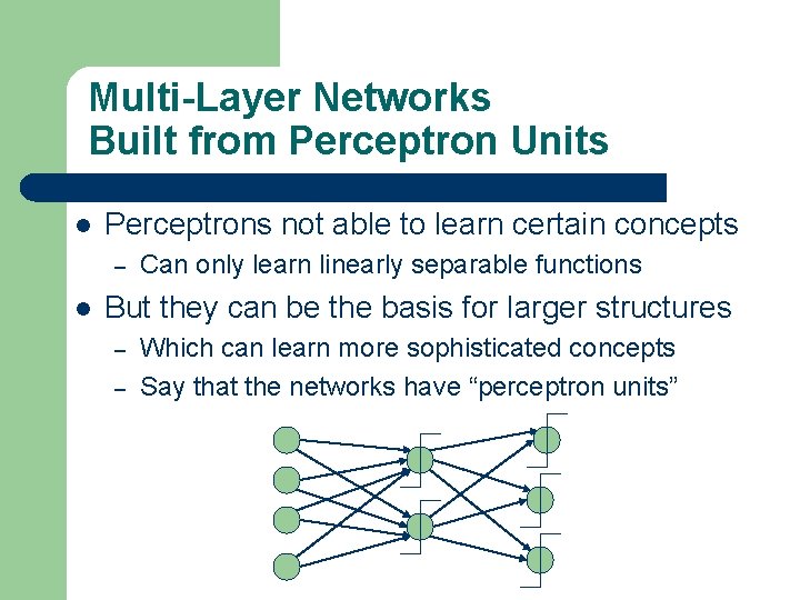
Multi-Layer Networks Built from Perceptron Units l Perceptrons not able to learn certain concepts – l Can only learn linearly separable functions But they can be the basis for larger structures – – Which can learn more sophisticated concepts Say that the networks have “perceptron units”

Problem With Perceptron Units l The learning rule relies on differential calculus – l Step functions aren’t differentiable – l Finding minima by differentiating, etc. They are not continuous at the threshold Alternative threshold function sought – – Must be differentiable Must be similar to step function l l i. e. , exhibit a threshold so that units can “fire” or not fire Sigmoid units used for backpropagation – There are other alternatives that are often used

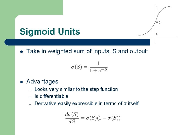
Sigmoid Units l Take in weighted sum of inputs, S and output: l Advantages: – – – Looks very similar to the step function Is differentiable Derivative easily expressible in terms of σ itself:

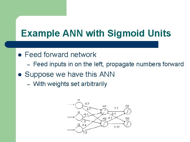
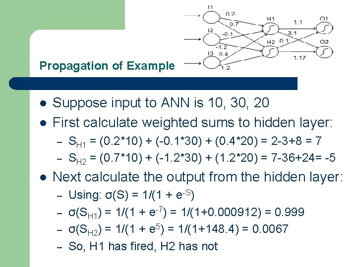
Example ANN with Sigmoid Units l Feed forward network – l Feed inputs in on the left, propagate numbers forward Suppose we have this ANN – With weights set arbitrarily

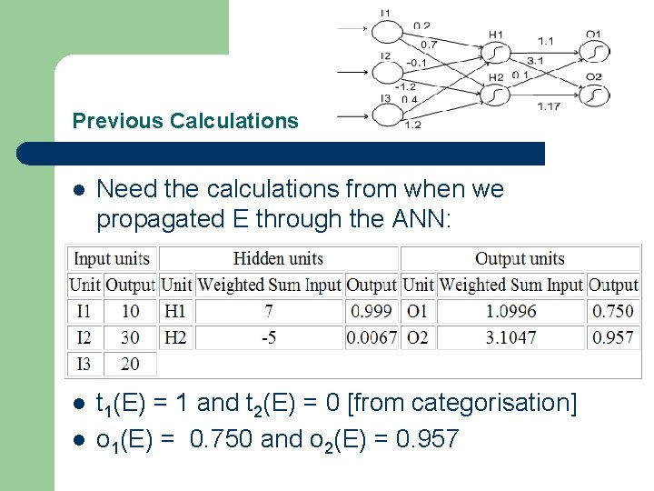
Propagation of Example l l Suppose input to ANN is 10, 30, 20 First calculate weighted sums to hidden layer: – – l SH 1 = (0. 2*10) + (-0. 1*30) + (0. 4*20) = 2 -3+8 = 7 SH 2 = (0. 7*10) + (-1. 2*30) + (1. 2*20) = 7 -36+24= -5 Next calculate the output from the hidden layer: – – Using: σ(S) = 1/(1 + e-S) σ(SH 1) = 1/(1 + e-7) = 1/(1+0. 000912) = 0. 999 σ(SH 2) = 1/(1 + e 5) = 1/(1+148. 4) = 0. 0067 So, H 1 has fired, H 2 has not

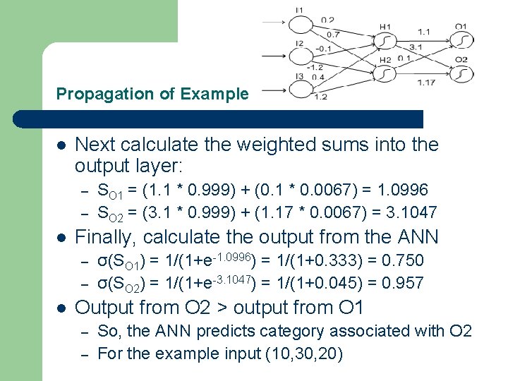
Propagation of Example l Next calculate the weighted sums into the output layer: – – l Finally, calculate the output from the ANN – – l SO 1 = (1. 1 * 0. 999) + (0. 1 * 0. 0067) = 1. 0996 SO 2 = (3. 1 * 0. 999) + (1. 17 * 0. 0067) = 3. 1047 σ(SO 1) = 1/(1+e-1. 0996) = 1/(1+0. 333) = 0. 750 σ(SO 2) = 1/(1+e-3. 1047) = 1/(1+0. 045) = 0. 957 Output from O 2 > output from O 1 – – So, the ANN predicts category associated with O 2 For the example input (10, 30, 20)

Backpropagation Learning Algorithm l Same task as in perceptrons – – l Learn a multi-layer ANN to correctly categorise unseen examples We’ll concentrate on ANNs with one hidden layer Overview of the routine – Fix architecture and sigmoid units within architecture l – Randomly assign weights to the whole network l – – i. e. , number of units in hidden layer; the way the input units represent example; the way the output units categorises examples Use small values (between – 0. 5 and 0. 5) Use each example in the set to retrain the weights Have multiple epochs (iterations through training set) l Until some termination condition is met (not necessarily 100% acc)

Weight Training Calculations (Overview) l Use notation wij to specify: – l l Look at the calculation with respect to example E Going to calculate a value Δij for each wij – l l And add Δij on to wij Do this by calculating error terms for each unit The error term for output units is found – l Weight between unit i and unit j And then this information is used to calculate the error terms for the hidden units So, the error is propagated back through the ANN

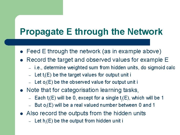
Propagate E through the Network l l Feed E through the network (as in example above) Record the target and observed values for example E – – – l Note that for categorisation learning tasks, – – l i. e. , determine weighted sum from hidden units, do sigmoid calc Let ti(E) be the target values for output unit i Let oi(E) be the observed value for output unit i Each ti(E) will be 0, except for a single tj(E), which will be 1 But oi(E) will be a real valued number between 0 and 1 Also record the outputs from the hidden units – Let hi(E) be the output from hidden unit i

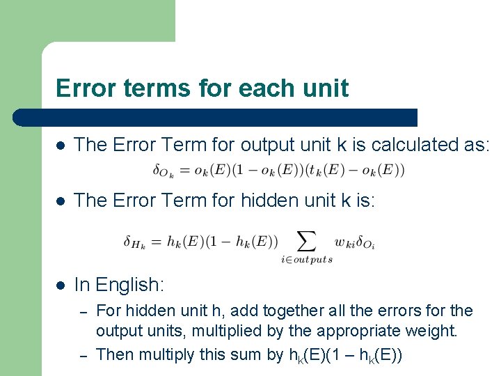
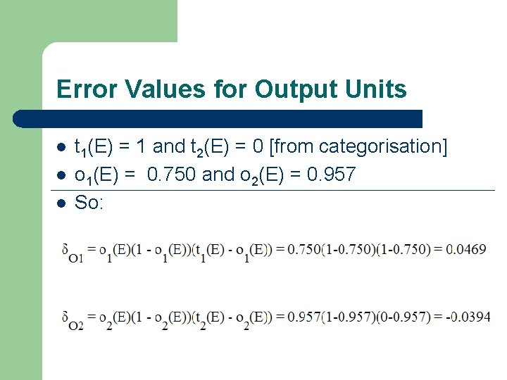
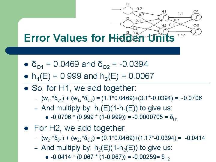
Error terms for each unit l The Error Term for output unit k is calculated as: l The Error Term for hidden unit k is: l In English: – – For hidden unit h, add together all the errors for the output units, multiplied by the appropriate weight. Then multiply this sum by hk(E)(1 – hk(E))

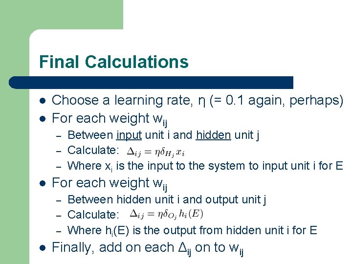
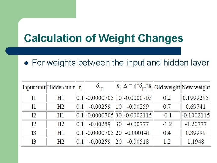
Final Calculations l l Choose a learning rate, η (= 0. 1 again, perhaps) For each weight wij – – – l Between input unit i and hidden unit j Calculate: Where xi is the input to the system to input unit i for E Between hidden unit i and output unit j Calculate: Where hi(E) is the output from hidden unit i for E Finally, add on each Δij on to wij

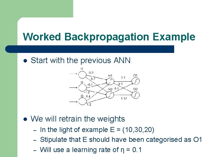
Worked Backpropagation Example l Start with the previous ANN l We will retrain the weights – – – In the light of example E = (10, 30, 20) Stipulate that E should have been categorised as O 1 Will use a learning rate of η = 0. 1

Previous Calculations l Need the calculations from when we propagated E through the ANN: l t 1(E) l = 1 and t 2(E) = 0 [from categorisation] o 1(E) = 0. 750 and o 2(E) = 0. 957

Error Values for Output Units l t 1(E) l l = 1 and t 2(E) = 0 [from categorisation] o 1(E) = 0. 750 and o 2(E) = 0. 957 So:

Error Values for Hidden Units l l l δO 1 = 0. 0469 and δO 2 = -0. 0394 h 1(E) = 0. 999 and h 2(E) = 0. 0067 So, for H 1, we add together: – (w 11*δ 01) + (w 12*δO 2) = (1. 1*0. 0469)+(3. 1*-0. 0394) = -0. 0706 – And multiply by: h 1(E)(1 -h 1(E)) to give us: l l -0. 0706 * (0. 999 * (1 -0. 999)) = -0. 0000705 = δH 1 For H 2, we add together: – (w 21*δ 01) + (w 22*δO 2) = (0. 1*0. 0469)+(1. 17*-0. 0394) = -0. 0414 – And multiply by: h 2(E)(1 -h 2(E)) to give us: l -0. 0414 * (0. 067 * (1 -0. 067)) = -0. 00259= δH 2

Calculation of Weight Changes l For weights between the input and hidden layer

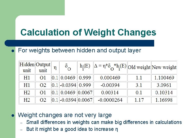
Calculation of Weight Changes l For weights between hidden and output layer l Weight changes are not very large – – Small differences in weights can make big differences in calculations But it might be a good idea to increase η

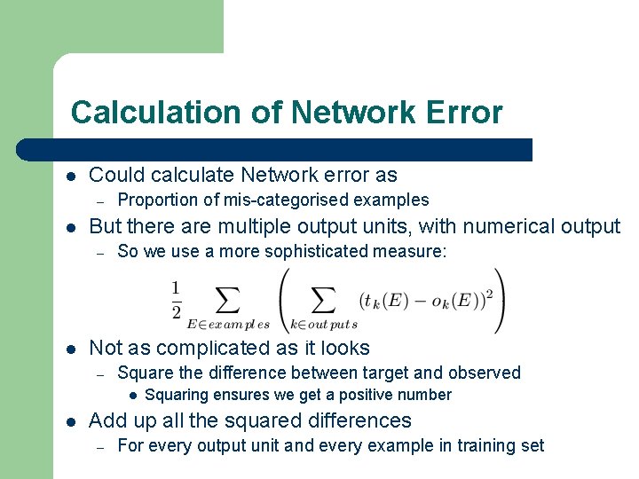
Calculation of Network Error l Could calculate Network error as – l But there are multiple output units, with numerical output – l Proportion of mis-categorised examples So we use a more sophisticated measure: Not as complicated as it looks – Square the difference between target and observed l l Squaring ensures we get a positive number Add up all the squared differences – For every output unit and every example in training set

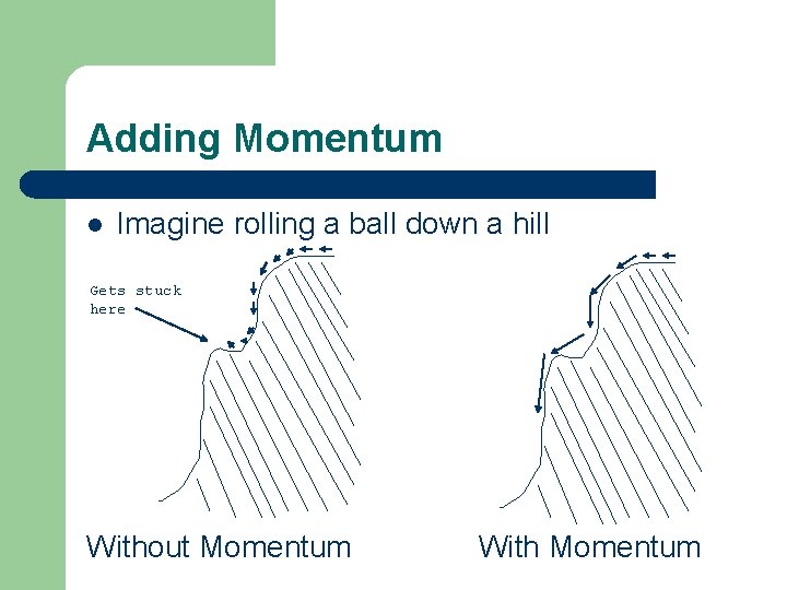
Problems with Local Minima l Backpropagation is gradient descent search – – Where the height of the hills is determined by error But there are many dimensions to the space l l Therefore backpropagation – l Can find its ways into local minima One partial solution: – Random re-start: learn lots of networks l – – l One for each weight in the network Starting with different random weight settings Can take best network Or can set up a “committee” of networks to categorise examples Another partial solution: Momentum

Adding Momentum l Imagine rolling a ball down a hill Gets stuck here Without Momentum With Momentum

Momentum in Backpropagation l For each weight – l In the current epoch – l Remember what was added in the previous epoch Add on a small amount of the previous Δ The amount is determined by – – The momentum parameter, denoted α α is taken to be between 0 and 1

How Momentum Works l If direction of the weight doesn’t change – – l Then the movement of search gets bigger The amount of additional extra is compounded in each epoch May mean that narrow local minima are avoided May also mean that the convergence rate speeds up Caution: – – May not have enough momentum to get out of local minima Also, too much momentum might carry search l Back out of the global minimum, into a local minimum

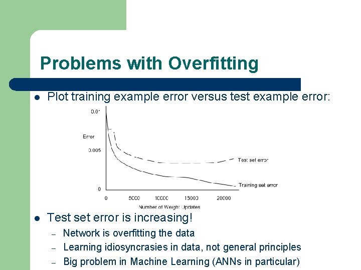
Problems with Overfitting l Plot training example error versus test example error: l Test set error is increasing! – – – Network is overfitting the data Learning idiosyncrasies in data, not general principles Big problem in Machine Learning (ANNs in particular)

Avoiding Overfitting l l Bad idea to use training set accuracy to terminate One alternative: Use a validation set – – – Hold back some of the training set during training Like a miniature test set (not used to train weights at all) If the validation set error stops decreasing, but the training set error continues decreasing l – Be careful, because validation set error could get into a local minima itself l l Then it’s likely that overfitting has started to occur, so stop Worthwhile running the training for longer, and wait and see Another alternative: use a weight decay factor – – Take a small amount off every weight after each epoch Networks with smaller weights aren’t as highly fine tuned (overfit)

Suitable Problems for ANNs l Examples and target categorisation – Can be expressed as real values l l Predictive accuracy is more important – Than understanding what the machine has learned l l Can take hours and days to train networks Execution of learned function must be quick – Learned networks can categorise very quickly l l Black box non-symbolic approach, not easy to digest Slow training times are OK – l ANNs are just fancy numerical functions Very useful in time critical situations (is that a tank, car or old lady? ) Error: ANNs are fairly robust to noise in data