Approximate Inference 2 Monte Carlo Markov Chain 1

Approximate Inference 2: Monte Carlo Markov Chain 1

MCMC Limitations of LW: • Evidence affects sampling only for nodes that are its descendants • For nondescendants, the weights account for the effect of the evidence • If evidence is at the leaves, we are sampling from the prior distribution (and not the posterior which is what we want)

MCMC Strategy used by MCMC • Generate a sequence of samples • Initial samples generated from the prior • Successive samples generated progressively closer to the posterior Applies to both directed and undirected models. We’ll use a distribution P defined in terms of a set of factors

Gibbs Sampling

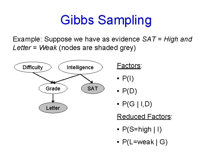
Gibbs Sampling Example: Suppose we have as evidence SAT = High and Letter = Weak (nodes are shaded grey) Difficulty Intelligence Factors: • P(I) Grade Letter SAT • P(D) • P(G | I, D) Reduced Factors: • P(S=high | I) • P(L=weak | G)

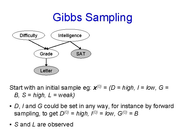
Gibbs Sampling Intelligence Difficulty Grade SAT Letter Start with an initial sample eg: x(0) = (D = high, I = low, G = B, S = high, L = weak) • D, I and G could be set in any way, for instance by forward sampling, to get D(0) = high, I(0) = low, G(0) = B • S and L are observed

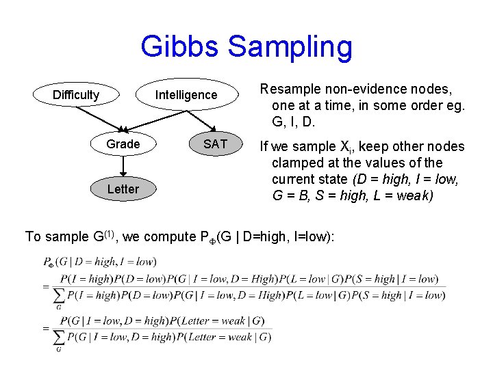
Gibbs Sampling Intelligence Difficulty Grade Letter SAT Resample non-evidence nodes, one at a time, in some order eg. G, I, D. If we sample Xi, keep other nodes clamped at the values of the current state (D = high, I = low, G = B, S = high, L = weak) To sample G(1), we compute P (G | D=high, I=low):

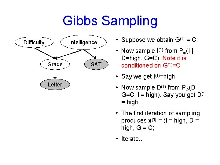
Gibbs Sampling Intelligence Difficulty Grade SAT • Suppose we obtain G(1) = C. • Now sample I(1) from P (I | D=high, G=C). Note it is conditioned on G(1)=C • Say we get I(1)=high Letter • Now sample D(1) from P (D | G=C, I = high). Say you get D(1) = high • The first iteration of sampling produces x(1) = (I = high, D = high, G = C) • Iterate. . .

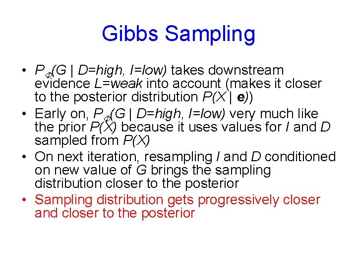
Gibbs Sampling • P (G | D=high, I=low) takes downstream evidence L=weak into account (makes it closer to the posterior distribution P(X | e)) • Early on, P (G | D=high, I=low) very much like the prior P(X) because it uses values for I and D sampled from P(X) • On next iteration, resampling I and D conditioned on new value of G brings the sampling distribution closer to the posterior • Sampling distribution gets progressively closer and closer to the posterior

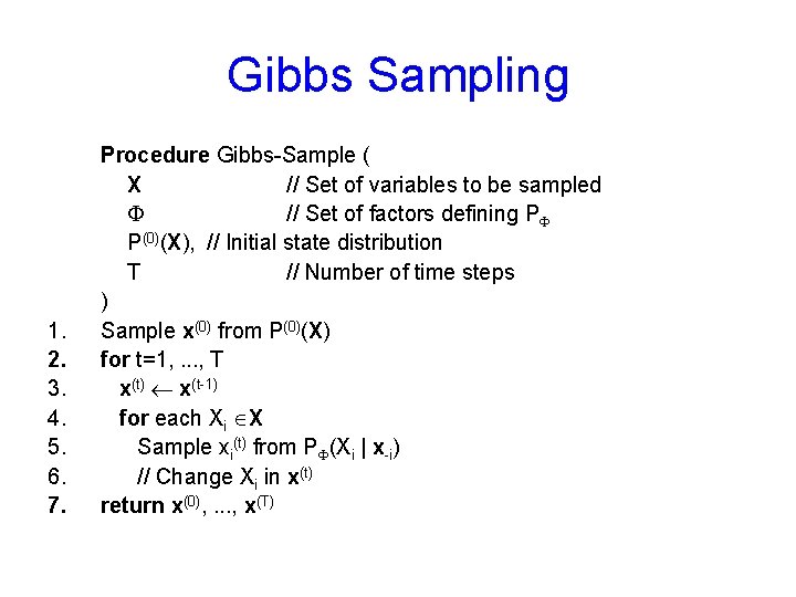
Gibbs Sampling 1. 2. 3. 4. 5. 6. 7. Procedure Gibbs-Sample ( X // Set of variables to be sampled // Set of factors defining P P(0)(X), // Initial state distribution T // Number of time steps ) Sample x(0) from P(0)(X) for t=1, . . . , T x(t) x(t-1) for each Xi X Sample xi(t) from P (Xi | x-i) // Change Xi in x(t) return x(0), . . . , x(T)

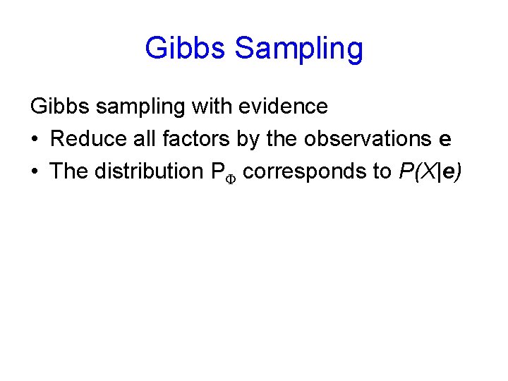
Gibbs Sampling Gibbs sampling with evidence • Reduce all factors by the observations e • The distribution P corresponds to P(X|e)

Markov Chains

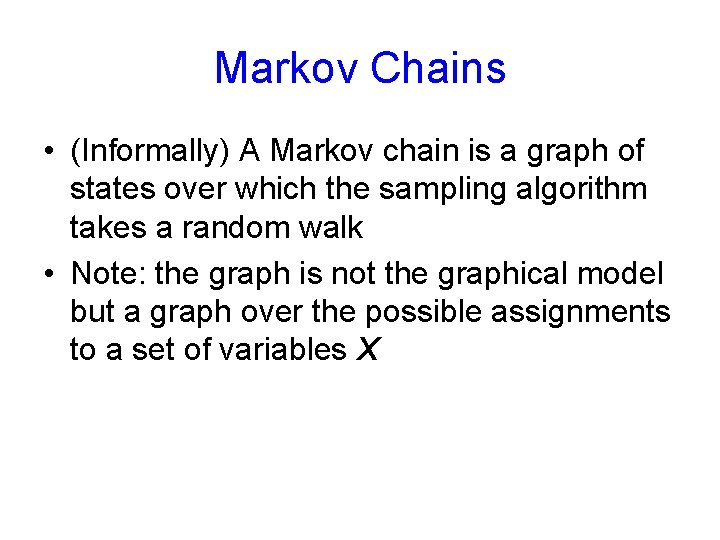
Markov Chains • (Informally) A Markov chain is a graph of states over which the sampling algorithm takes a random walk • Note: the graph is not the graphical model but a graph over the possible assignments to a set of variables X

Markov Chains • A Markov chain is defined via a state space Val(X) and a model that defines, for every state x Val(X) a next-state distribution over Val(X). • More precisely, the transition model T specifies for each pair of states x, x’ the probability T(x x’) of going from x to x’. • A homogeneous Markov chain is one where the system dynamics do not change over time

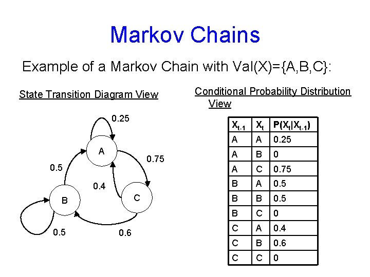
Markov Chains Example of a Markov Chain with Val(X)={A, B, C}: State Transition Diagram View 0. 25 A 0. 75 0. 4 C B 0. 5 0. 6 Conditional Probability Distribution View Xt-1 Xt P(Xt|Xt-1) A A 0. 25 A B 0 A C 0. 75 B A 0. 5 B B 0. 5 B C 0 C A 0. 4 C B 0. 6 C C 0

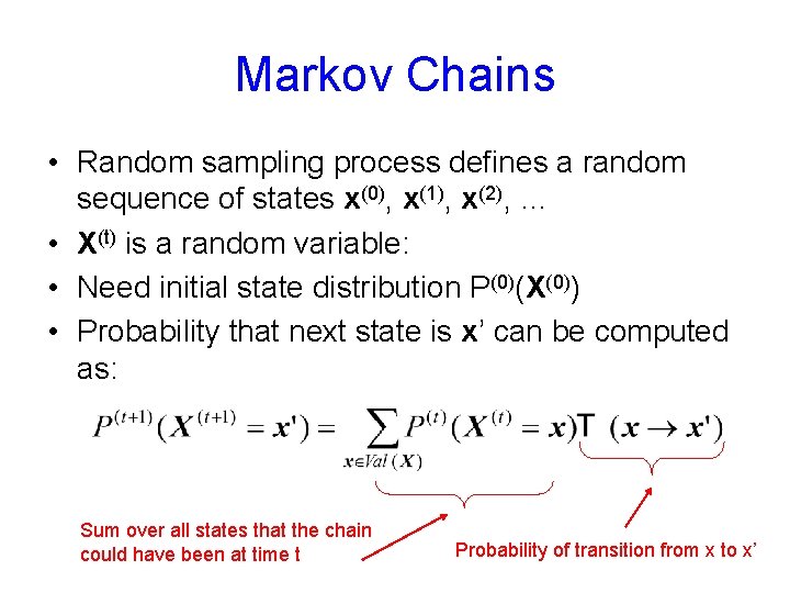
Markov Chains • Random sampling process defines a random sequence of states x(0), x(1), x(2), … • X(t) is a random variable: • Need initial state distribution P(0)(X(0)) • Probability that next state is x’ can be computed as: Sum over all states that the chain could have been at time t Probability of transition from x to x’

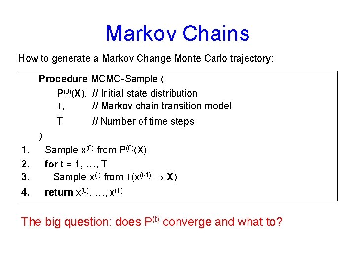
Markov Chains How to generate a Markov Change Monte Carlo trajectory: Procedure MCMC-Sample ( P(0)(X), // Initial state distribution T, // Markov chain transition model T // Number of time steps ) 1. 2. 3. Sample x(0) from P(0)(X) for t = 1, …, T Sample x(t) from T(x(t-1) X) 4. return x(0), …, x(T) The big question: does P(t) converge and what to?

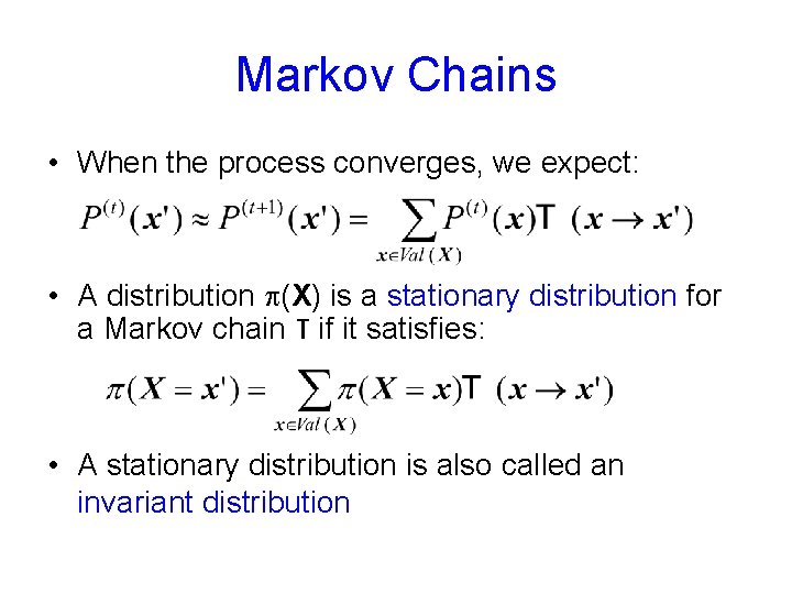
Markov Chains • When the process converges, we expect: • A distribution (X) is a stationary distribution for a Markov chain T if it satisfies: • A stationary distribution is also called an invariant distribution

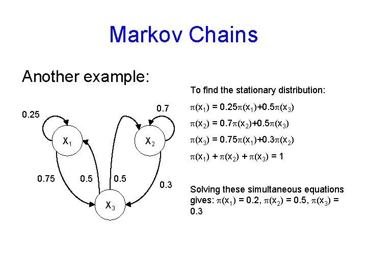
Markov Chains Another example: To find the stationary distribution: 0. 7 0. 25 (x 1) = 0. 25 (x 1)+0. 5 (x 3) (x 2) = 0. 7 (x 2)+0. 5 (x 3) X 1 (x 3) = 0. 75 (x 1)+0. 3 (x 2) X 2 (x 1) + (x 2) + (x 3) = 1 0. 75 0. 5 X 3 0. 3 Solving these simultaneous equations gives: (x 1) = 0. 2, (x 2) = 0. 5, (x 3) = 0. 3

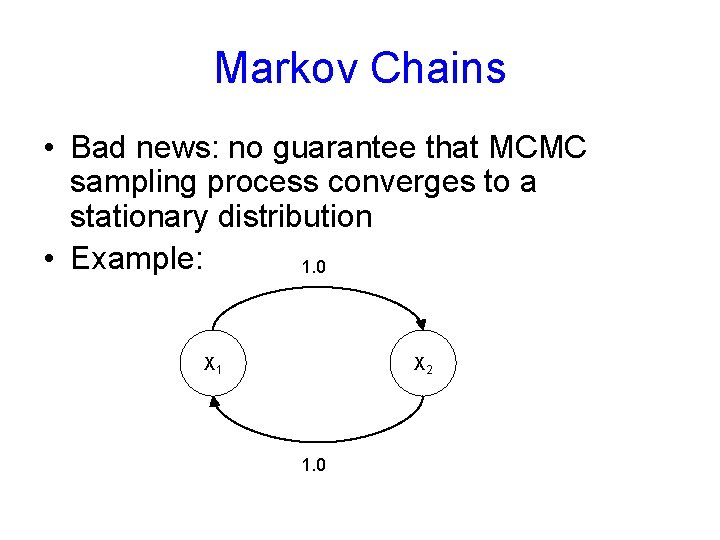
Markov Chains • Bad news: no guarantee that MCMC sampling process converges to a stationary distribution • Example: 1. 0 X 1 X 2 1. 0

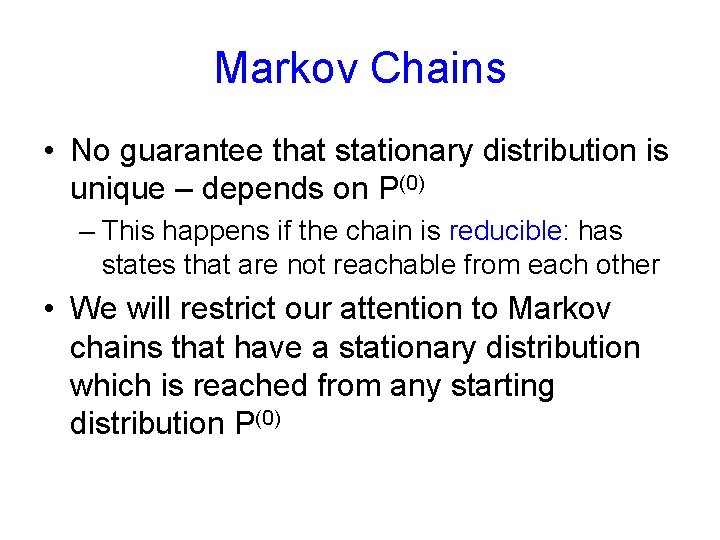
Markov Chains • No guarantee that stationary distribution is unique – depends on P(0) – This happens if the chain is reducible: has states that are not reachable from each other • We will restrict our attention to Markov chains that have a stationary distribution which is reached from any starting distribution P(0)

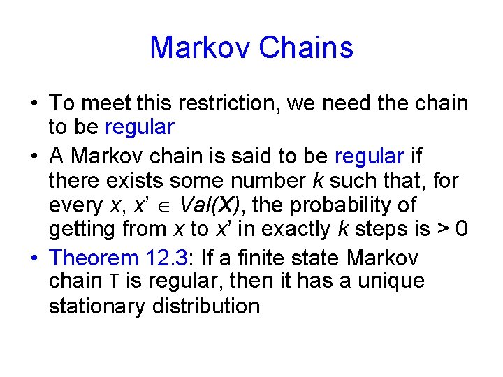
Markov Chains • To meet this restriction, we need the chain to be regular • A Markov chain is said to be regular if there exists some number k such that, for every x, x’ Val(X), the probability of getting from x to x’ in exactly k steps is > 0 • Theorem 12. 3: If a finite state Markov chain T is regular, then it has a unique stationary distribution

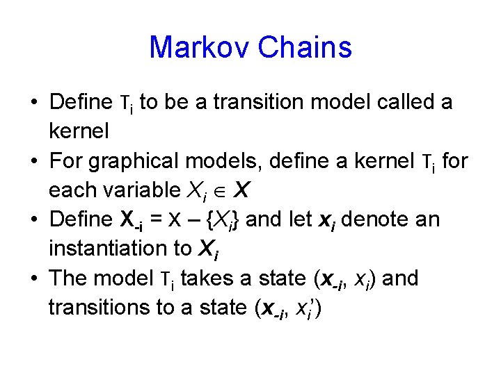
Markov Chains • Define Ti to be a transition model called a kernel • For graphical models, define a kernel Ti for each variable Xi X • Define X-i = X – {Xi} and let xi denote an instantiation to Xi • The model Ti takes a state (x-i, xi) and transitions to a state (x-i, xi’)

Gibbs Sampling Revisited

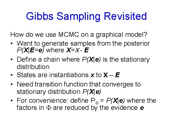
Gibbs Sampling Revisited How do we use MCMC on a graphical model? • Want to generate samples from the posterior P(X|E=e) where X=X - E • Define a chain where P(X|e) is the stationary distribution • States are instantiations x to X – E • Need transition function that converges to stationary distribution P(X|e) • For convenience: define P = P(X|e) where the factors in are reduced by the evidence e

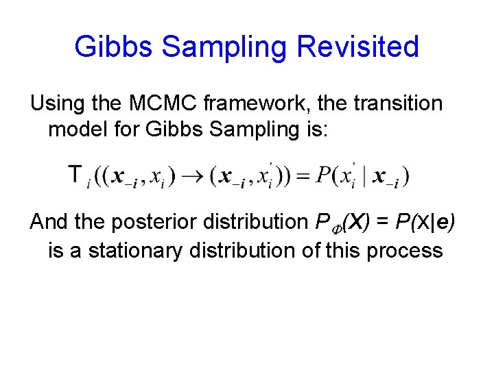
Gibbs Sampling Revisited Using the MCMC framework, the transition model for Gibbs Sampling is: And the posterior distribution P (X) = P(X|e) is a stationary distribution of this process

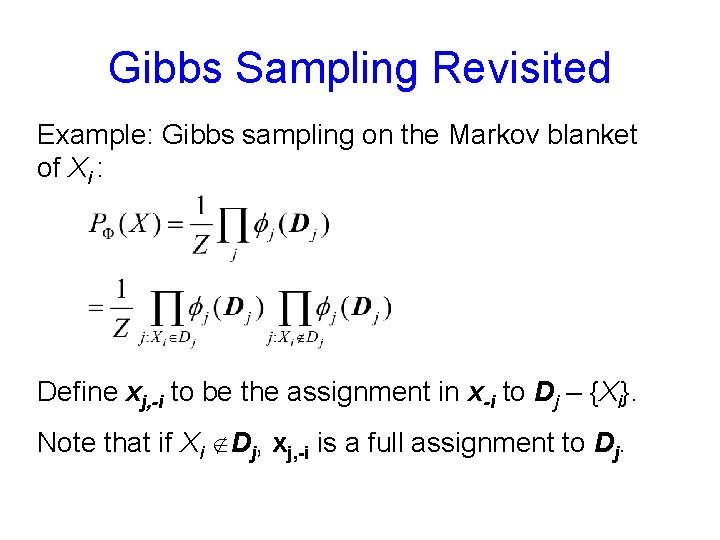
Gibbs Sampling Revisited Example: Gibbs sampling on the Markov blanket of Xi : Define xj, -i to be the assignment in x-i to Dj – {Xi}. Note that if Xi Dj, xj, -i is a full assignment to Dj.

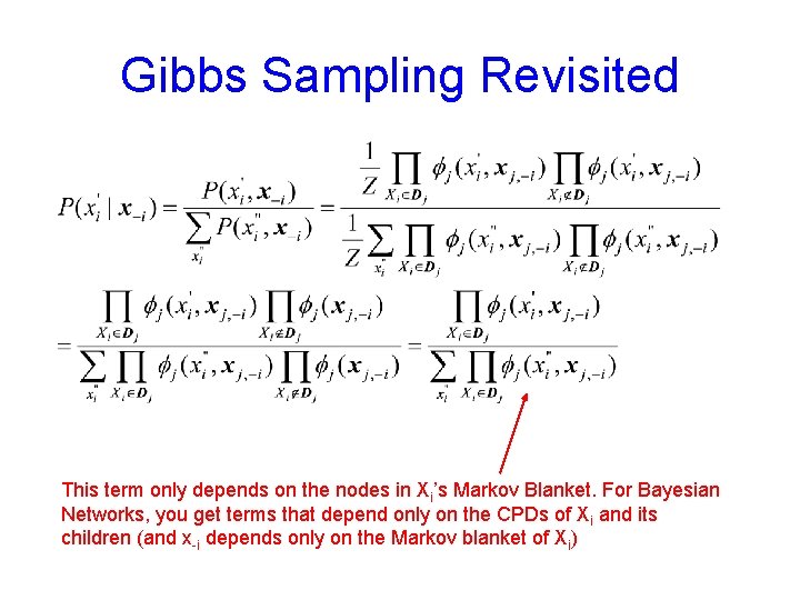
Gibbs Sampling Revisited This term only depends on the nodes in Xi’s Markov Blanket. For Bayesian Networks, you get terms that depend only on the CPDs of Xi and its children (and x-i depends only on the Markov blanket of Xi)

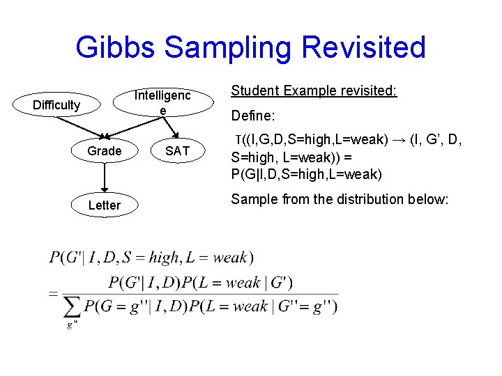
Gibbs Sampling Revisited Intelligenc e Difficulty Grade Letter SAT Student Example revisited: Define: T((I, G, D, S=high, L=weak) → (I, G’, D, S=high, L=weak)) = P(G|I, D, S=high, L=weak) Sample from the distribution below:

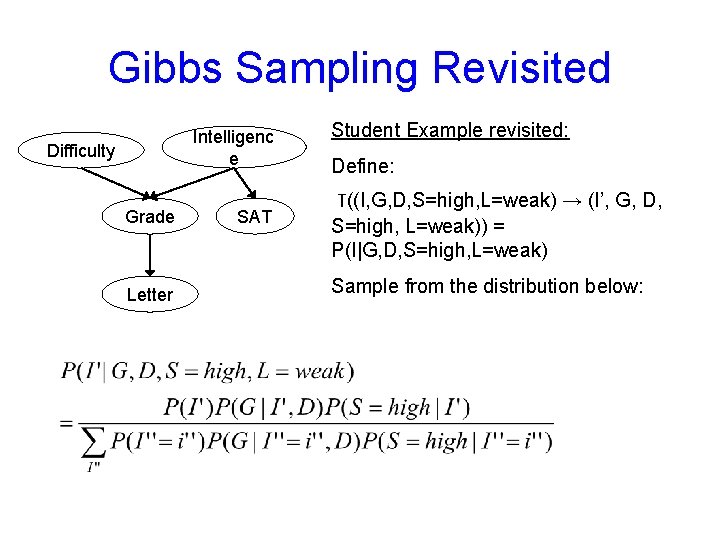
Gibbs Sampling Revisited Intelligenc e Difficulty Grade Letter SAT Student Example revisited: Define: T((I, G, D, S=high, L=weak) → (I’, G, D, S=high, L=weak)) = P(I|G, D, S=high, L=weak) Sample from the distribution below:

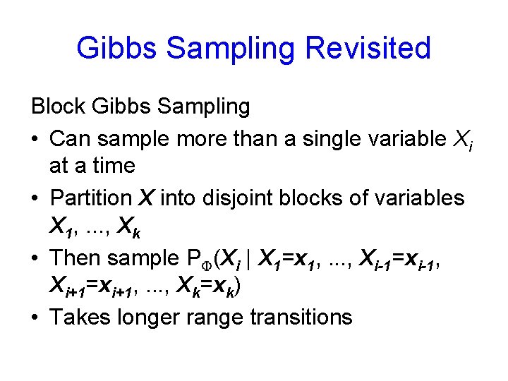
Gibbs Sampling Revisited Block Gibbs Sampling • Can sample more than a single variable Xi at a time • Partition X into disjoint blocks of variables X 1, . . . , Xk • Then sample P (Xi | X 1=x 1, . . . , Xi-1=xi-1, Xi+1=xi+1, . . . , Xk=xk) • Takes longer range transitions

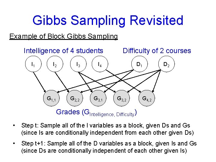
Gibbs Sampling Revisited Example of Block Gibbs Sampling Intelligence of 4 students I 1 I 2 I 3 I 4 G 1, 1 G 2, 2 G 3, 1 Difficulty of 2 courses D 1 G 3, 2 D 2 G 4, 2 Grades (GIntelligence, Difficulty) • Step t: Sample all of the I variables as a block, given Ds and Gs (since Is are conditionally independent from each other given Ds) • Step t+1: Sample all of the D variables as a block, given Is and Gs (since Ds are conditionally independent of each other given Is)

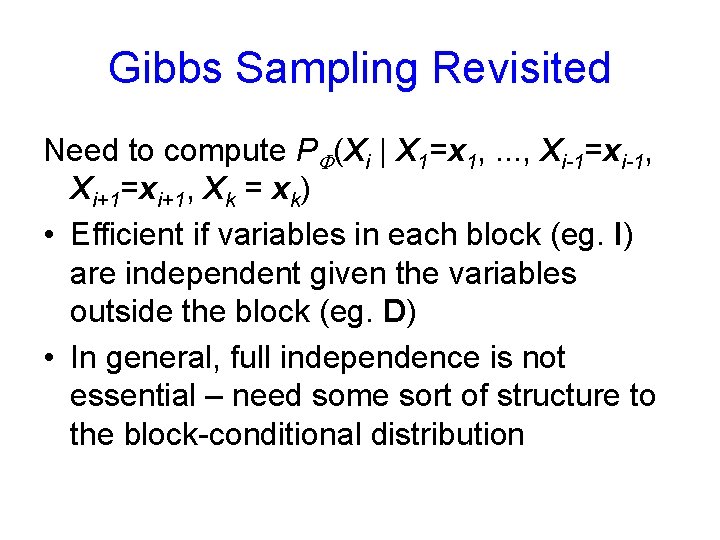
Gibbs Sampling Revisited Need to compute P (Xi | X 1=x 1, . . . , Xi-1=xi-1, Xi+1=xi+1, Xk = xk) • Efficient if variables in each block (eg. I) are independent given the variables outside the block (eg. D) • In general, full independence is not essential – need some sort of structure to the block-conditional distribution

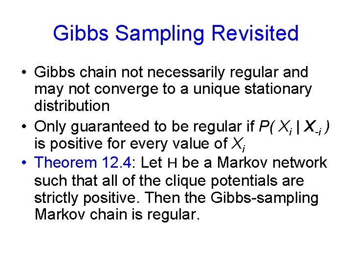
Gibbs Sampling Revisited • Gibbs chain not necessarily regular and may not converge to a unique stationary distribution • Only guaranteed to be regular if P( Xi | X-i ) is positive for every value of Xi • Theorem 12. 4: Let H be a Markov network such that all of the clique potentials are strictly positive. Then the Gibbs-sampling Markov chain is regular.

Gibbs Sampling Revisited • But many examples of nonpositive distributions where Gibbs chain is regular • Some regular chains may even take a long time to converge to the stationary distribution