Air Pollution Meteorology General considerations on the atmospheric

Air Pollution Meteorology • • • General considerations on the atmospheric planetary boundary layer Vertical motions of air parcels Winds and turbulence Heat transfer Local circulations

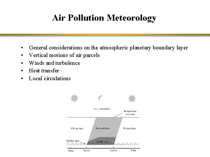
The Atmospheric Planetary Boundary Layer The atmospheric planetary boundary layer (PBL) is defined as the atmospheric layer that is influenced by the Earth’s surface. – From a dynamic viewpoint, it is the layer where the flow is influenced by the surface, either because of solely mechanical effects (terrain roughness, presence of buildings…), or indirectly because of thermal effects (evaporation, urban heat island). – From a heat transfer viewpoint, it is the layer where the diurnal variation of the solar radiation can be observed (temperature variation for example). The PBL height varies as a function of terrain and solar radiation – A few hundred meters (or less) when solar radiation is low (e. g. , winter) – A few thousand meters when solar radiation is intense (e. g. , midday in summer)

Surface Layer The surface layer is defined as the atmospheric layer near the surface where the vertical fluxes of momentum, sensible heat, and latent heat are constant and equal to their value at the surface. The surface layer is at most 10 % of the height of the PBL.

Free Troposphere The free troposphere is above the PBL. - It is not influenced by the interactions with the Earth’s surface. - It is typically not taken into account when modeling air pollution at local or urban scales. - It must be taken into account when modeling air pollution at regional, continental, or global scales, because air pollutants can be transported above the PBL over long distances.

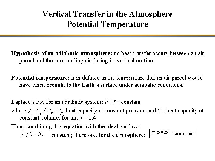
Vertical Transfer in the Atmosphere Potential Temperature Hypothesis of an adiabatic atmosphere: no heat transfer occurs between an air parcel and the surrounding air during its vertical motion. Potential temperature: It is defined as the temperature that an air parcel would have when brought to the Earth’s surface under adiabatic conditions. Laplace’s law for an adiabatic system: P Vg = constant where g = Cp / Cv ; Cp: heat capacity at constant pressure and Cv: heat capacity at constant volume; for air: g = 1. 4 Thus, combining this equation with the ideal gas law: -0. 29 = constant T P((1 – g)/g) = constant; therefore, for the atmosphere: T P

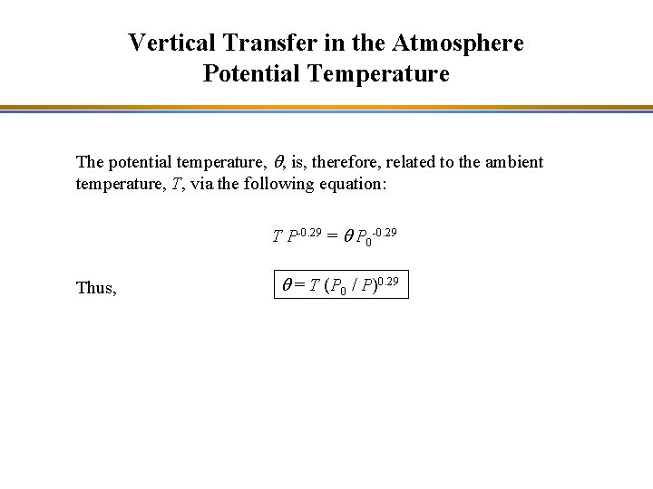
Vertical Transfer in the Atmosphere Potential Temperature The potential temperature, q, is, therefore, related to the ambient temperature, T, via the following equation: T P-0. 29 = q P 0 -0. 29 Thus, q = T (P 0 / P)0. 29

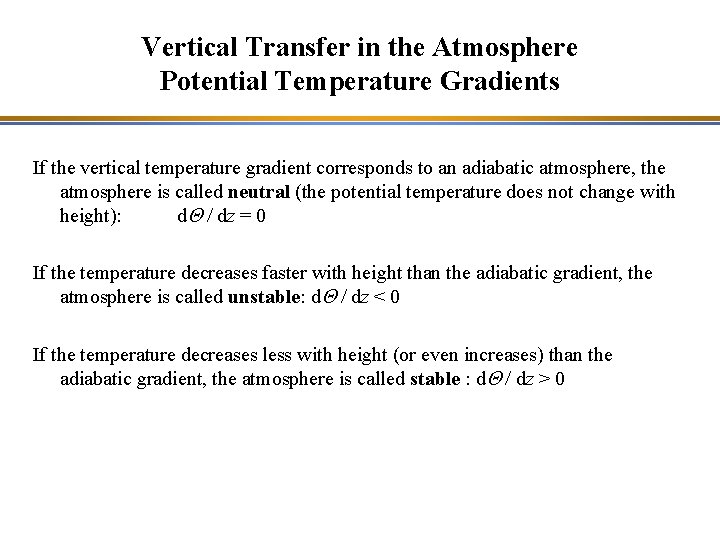
Vertical Transfer in the Atmosphere Potential Temperature Gradients If the vertical temperature gradient corresponds to an adiabatic atmosphere, the atmosphere is called neutral (the potential temperature does not change with height): d. Q / dz = 0 If the temperature decreases faster with height than the adiabatic gradient, the atmosphere is called unstable: d. Q / dz < 0 If the temperature decreases less with height (or even increases) than the adiabatic gradient, the atmosphere is called stable : d. Q / dz > 0

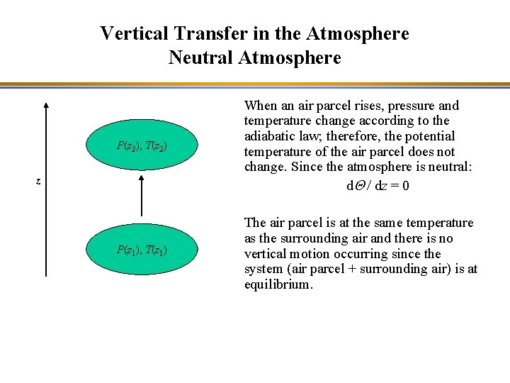
Vertical Transfer in the Atmosphere Neutral Atmosphere P(z 2), T(z 2) When an air parcel rises, pressure and temperature change according to the adiabatic law; therefore, the potential temperature of the air parcel does not change. Since the atmosphere is neutral: d. Q / dz = 0 P(z 1), T(z 1) The air parcel is at the same temperature as the surrounding air and there is no vertical motion occurring since the system (air parcel + surrounding air) is at equilibrium. z

Vertical Transfer in the Atmosphere Stable Atmosphere P(z 2), T(z 2) When an air parcel rises, pressure and temperature change according to the adiabatic law; therefore, the potential temperature of the air parcel does not change. Since the atmosphere is stable: d. Q / dz > 0 P(z 1), T(z 1) The air parcel has a temperature, which is lower than that of the surrounding air; to get back to equilibrium, the air parcel will move downward (since it is denser than the surrounding air). z A stable atmosphere suppresses vertical motions of air parcels.

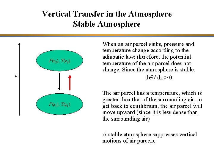
Vertical Transfer in the Atmosphere Stable Atmosphere P(z 2), T(z 2) When an air parcel sinks, pressure and temperature change according to the adiabatic law; therefore, the potential temperature of the air parcel does not change. Since the atmosphere is stable: d. Q / dz > 0 P(z 1), T(z 1) The air parcel has a temperature, which is greater than that of the surrounding air; to get back to equilibrium, the air parcel will move upward (since it is less dense than the surrounding air) z A stable atmosphere suppresses vertical motions of air parcels.

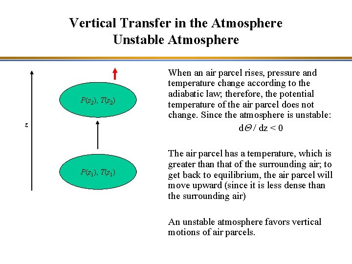
Vertical Transfer in the Atmosphere Unstable Atmosphere P(z 2), T(z 2) When an air parcel rises, pressure and temperature change according to the adiabatic law; therefore, the potential temperature of the air parcel does not change. Since the atmosphere is unstable: d. Q / dz < 0 P(z 1), T(z 1) The air parcel has a temperature, which is greater than that of the surrounding air; to get back to equilibrium, the air parcel will move upward (since it is less dense than the surrounding air) z An unstable atmosphere favors vertical motions of air parcels.

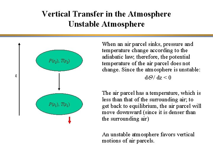
Vertical Transfer in the Atmosphere Unstable Atmosphere P(z 2), T(z 2) When an air parcel sinks, pressure and temperature change according to the adiabatic law; therefore, the potential temperature of the air parcel does not change. Since the atmosphere is unstable: d. Q / dz < 0 P(z 1), T(z 1) The air parcel has a temperature, which is less than that of the surrounding air; to get back to equilibrium, the air parcel will move downward (since it is denser than the surrounding air) z An unstable atmosphere favors vertical motions of air parcels.

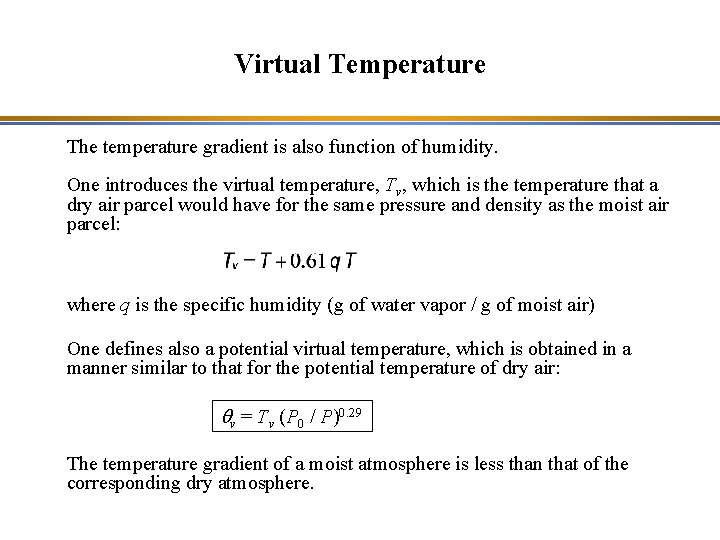
Virtual Temperature The temperature gradient is also function of humidity. One introduces the virtual temperature, Tv, which is the temperature that a dry air parcel would have for the same pressure and density as the moist air parcel: where q is the specific humidity (g of water vapor / g of moist air) One defines also a potential virtual temperature, which is obtained in a manner similar to that for the potential temperature of dry air: qv = Tv (P 0 / P)0. 29 The temperature gradient of a moist atmosphere is less than that of the corresponding dry atmosphere.

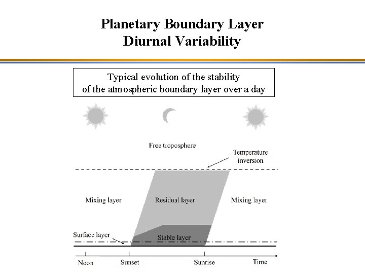
Planetary Boundary Layer Diurnal Variability Typical evolution of the stability of the atmospheric boundary layer over a day

Winds in the Free Troposphere The acceleration of an air parcel is proportional to the pressure gradient. Therefore, the wind results from a pressure difference between two locations: a steep pressure gradient leads to a strong wind due to the acceleration that results from that pressure gradient. The direction of the air flow is, in its simplest form, from the high pressure area toward the low pressure area. However, there are other forces (true or virtual) that affect wind direction.

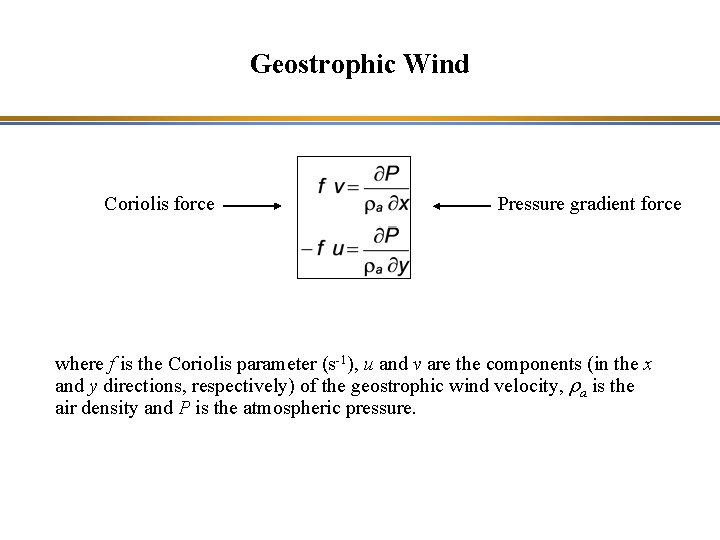
Geostrophic Wind Coriolis force Pressure gradient force where f is the Coriolis parameter (s-1), u and v are the components (in the x and y directions, respectively) of the geostrophic wind velocity, ra is the air density and P is the atmospheric pressure.

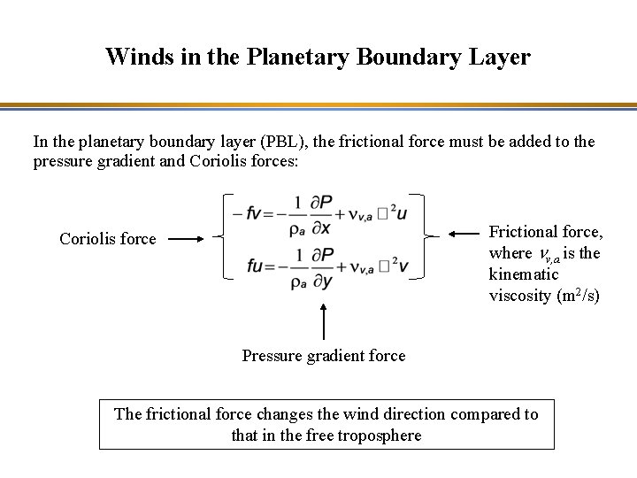
Winds in the Planetary Boundary Layer In the planetary boundary layer (PBL), the frictional force must be added to the pressure gradient and Coriolis forces: Frictional force, where nv, a is the kinematic viscosity (m 2/s) Coriolis force Pressure gradient force The frictional force changes the wind direction compared to that in the free troposphere

Winds in the Planetary Boundary Layer The Ekman Spiral The change in wind direction from the surface to the free troposphere is called the Ekman spiral (wind shear). The wind direction near the surface results from the balance among the pressure gradient, Coriolis, and frictional forces. The wind direction at the top of the PBL is that of the geostrophic wind, i. e. , it results from the balance between the pressure gradient and Coriolis forces.

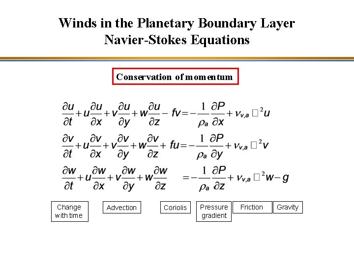
Winds in the Planetary Boundary Layer Navier-Stokes Equations The atmospheric flow is governed by the Navier-Stokes equations, which represent the conservation of momentum in a fluid. The atmosphere is considered to be a Newtonian fluid, i. e. , it has low viscosity. Air is a compressible fluid (as opposed for example to water). However, one introduces local hypotheses related to air being incompressible, which implies that its density is constant. - Anelastic hypothesis: the air density is constant at a given altitude (for example in a given numerical model layer). - Boussinesq hypothesis: the air density is constant, except when it is present in a term that includes the gravitational constant; this hypothesis applies to the planetary boundary layer.

Winds in the Planetary Boundary Layer Navier-Stokes Equations Conservation of momentum Change with time Advection Coriolis Pressure gradient Friction Gravity

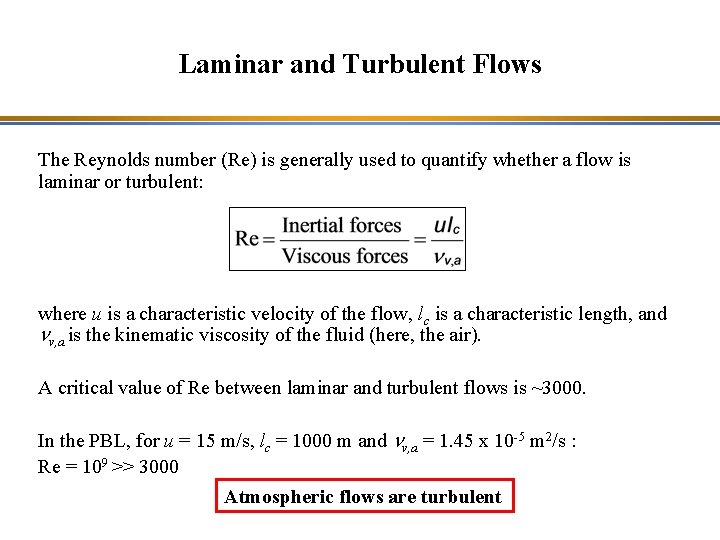
Laminar and Turbulent Flows The Reynolds number (Re) is generally used to quantify whether a flow is laminar or turbulent: where u is a characteristic velocity of the flow, lc is a characteristic length, and nv, a is the kinematic viscosity of the fluid (here, the air). A critical value of Re between laminar and turbulent flows is ~3000. In the PBL, for u = 15 m/s, lc = 1000 m and nv, a = 1. 45 x 10 -5 m 2/s : Re = 109 >> 3000 Atmospheric flows are turbulent

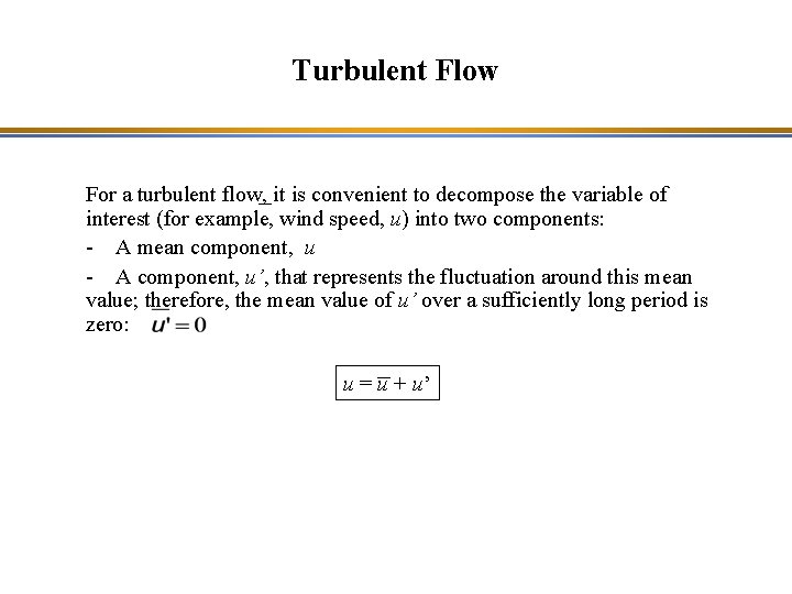
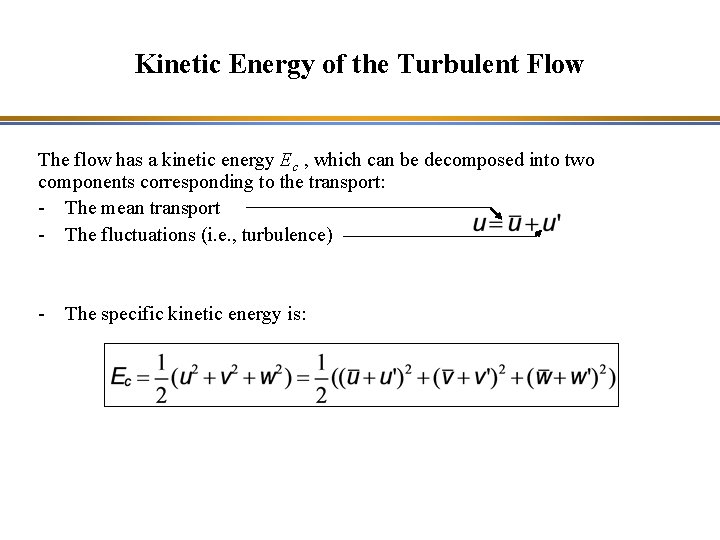
Turbulent Flow For a turbulent flow, it is convenient to decompose the variable of interest (for example, wind speed, u) into two components: - A mean component, u - A component, u’, that represents the fluctuation around this mean value; therefore, the mean value of u’ over a sufficiently long period is zero: u = u + u’

Kinetic Energy of Turbulent Flow The transfer of the kinetic energy of a turbulent flow occurs from the mean flow toward the turbulent eddies, cascading from the large eddies toward the smallest ones, and so on until the corresponding kinetic energy is converted to thermal energy via molecular viscosity. « Big whirls have little whirls that feed on their velocity and little whirls have lesser whirls and so on to viscosity » L. F. Richardson (1881 -1953)

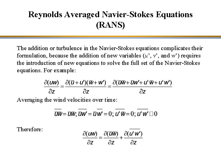
Reynolds Averaged Navier-Stokes Equations (RANS) The addition or turbulence in the Navier-Stokes equations complicates their formulation, because the addition of new variables (u’, v’, and w’) requires the introduction of new equations to solve the full set of the Navier-Stokes equations. For example: Averaging the wind velocities over time: Therefore:

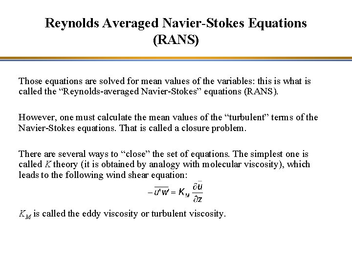
Reynolds Averaged Navier-Stokes Equations (RANS) Those equations are solved for mean values of the variables: this is what is called the “Reynolds-averaged Navier-Stokes” equations (RANS). However, one must calculate the mean values of the “turbulent” terms of the Navier-Stokes equations. That is called a closure problem. There are several ways to “close” the set of equations. The simplest one is called K theory (it is obtained by analogy with molecular viscosity), which leads to the following wind shear equation: KM is called the eddy viscosity or turbulent viscosity.

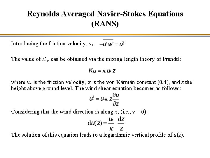
Reynolds Averaged Navier-Stokes Equations (RANS) Introducing the friction velocity, u*: The value of KM can be obtained via the mixing length theory of Prandtl: where u* is the friction velocity, k is the von Kármán constant (0. 4), and z the height above ground level. The wind shear equation becomes as follows: Considering that the wind direction is along x, (i. e. , v = 0): The solution of this equation leads to a logarithmic vertical profile of u(z).

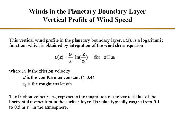
Winds in the Planetary Boundary Layer Vertical Profile of Wind Speed This vertical wind profile in the planetary boundary layer, u(z), is a logarithmic function, which is obtained by integration of the wind shear equation: where u* is the friction velocity k is the von Kármán constant (≈ 0. 4) z 0 is the roughness length The friction velocity, u*, represents the magnitude of the vertical flux of the horizontal momentum in the surface layer. Its value typically ranges from 0. 1 to 0. 5 m s-1 in the atmosphere.

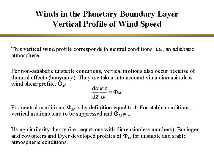
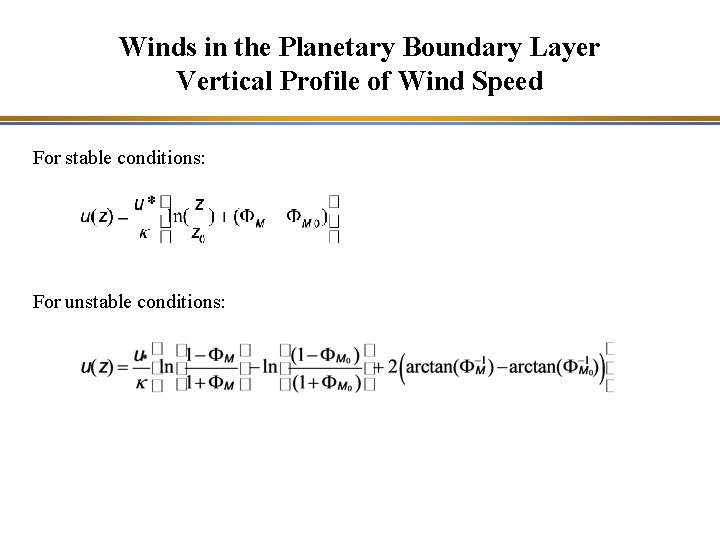
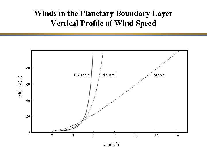
Winds in the Planetary Boundary Layer Vertical Profile of Wind Speed This vertical wind profile corresponds to neutral conditions, i. e. , an adiabatic atmosphere. For non-adiabatic unstable conditions, vertical motions also occur because of thermal effects (buoyancy). They are taken into account via a dimensionless wind shear profile, FM. For neutral conditions, FM is by definition equal to 1. For stable conditions, vertical motions tend to be suppressed and FM ≠ 1. Using similarity theory (i. e. , equations with dimensionless numbers), Businger and coworkers and Dyer developed profiles of FM for unstable and stable atmospheric conditions.

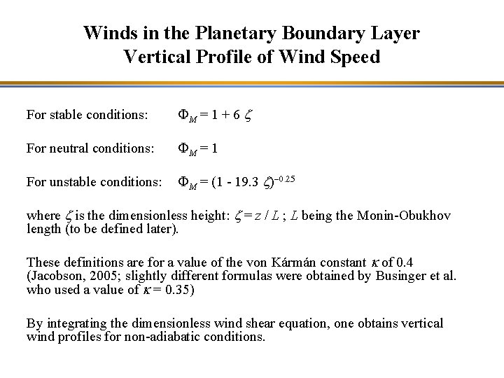
Winds in the Planetary Boundary Layer Vertical Profile of Wind Speed For stable conditions: FM = 1 + 6 z For neutral conditions: FM = 1 For unstable conditions: FM = (1 - 19. 3 z)-0. 25 where z is the dimensionless height: z = z / L ; L being the Monin-Obukhov length (to be defined later). These definitions are for a value of the von Kármán constant k of 0. 4 (Jacobson, 2005; slightly different formulas were obtained by Businger et al. who used a value of k = 0. 35) By integrating the dimensionless wind shear equation, one obtains vertical wind profiles for non-adiabatic conditions.

Winds in the Planetary Boundary Layer Vertical Profile of Wind Speed For stable conditions: For unstable conditions:

Winds in the Planetary Boundary Layer Vertical Profile of Wind Speed

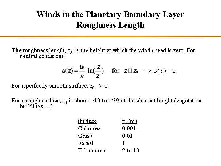
Winds in the Planetary Boundary Layer Roughness Length The roughness length, z 0, is the height at which the wind speed is zero. For neutral conditions: => u(z 0) = 0 For a perfectly smooth surface: z 0 => 0. For a rough surface, z 0 is about 1/10 to 1/30 of the element height (vegetation, buildings, …). Surface Calm sea Grass Forest Urban area z 0 (m) 0. 001 0. 01 1 2 to 10

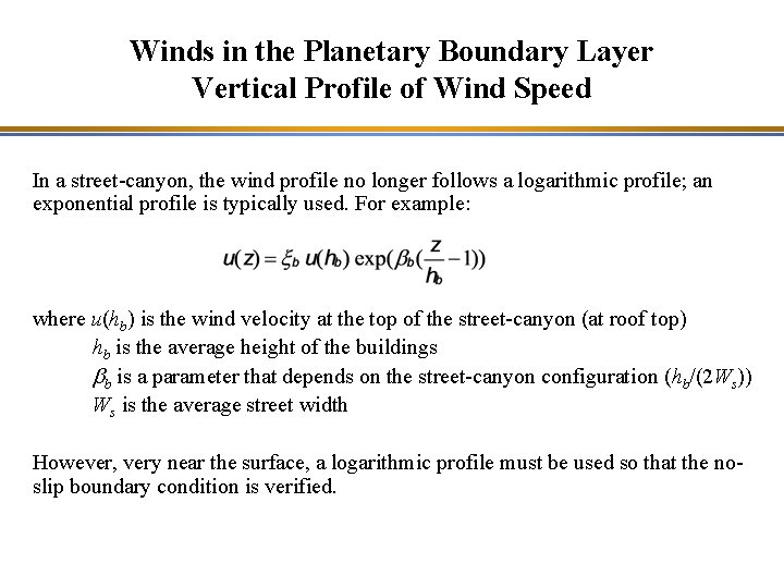
Winds in the Planetary Boundary Layer Vertical Profile of Wind Speed In a street-canyon, the wind profile no longer follows a logarithmic profile; an exponential profile is typically used. For example: where u(hb) is the wind velocity at the top of the street-canyon (at roof top) hb is the average height of the buildings bb is a parameter that depends on the street-canyon configuration (hb/(2 Ws)) Ws is the average street width However, very near the surface, a logarithmic profile must be used so that the noslip boundary condition is verified.

Kinetic Energy of the Turbulent Flow The flow has a kinetic energy Ec , which can be decomposed into two components corresponding to the transport: - The mean transport - The fluctuations (i. e. , turbulence) - The specific kinetic energy is:

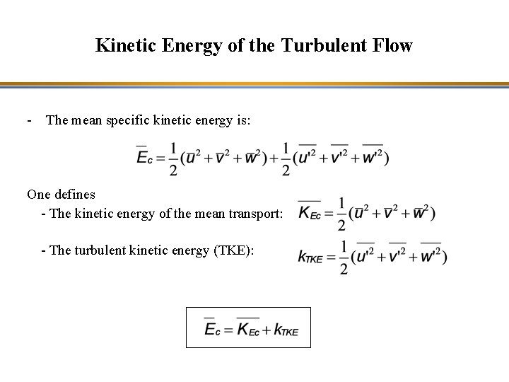
Kinetic Energy of the Turbulent Flow - The mean specific kinetic energy is: One defines - The kinetic energy of the mean transport: - The turbulent kinetic energy (TKE):

Navier-Stokes Equations Other Closure Approaches than K Theory More advanced closure models have been developed: - k-e model: it takes into account the dissipation of the turbulent energy via two additional equations that relate the turbulent kinetic energy (k) to its dissipation rate (e) - k-w model: it also takes into account the dissipation of the turbulent kinetic energy (k), but it uses the specific dissipation rate (w), which is the dissipation rate per unit of TKE. Even more advanced models use more detailed representation of turbulence: - « Large eddy simulation » (LES): use of parameterizations to represent the spectrum of the large turbulent eddies - « Direct numerical simulation » (DNS): the simulation is even more detailed (no parameterization of turbulence) To add a better representation of turbulence in a model may improve the results, but it will increase the computational time significantly.

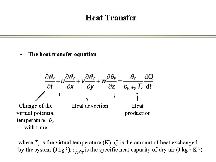
Heat Transfer - The heat transfer equation Zone Change of the virtual potential temperature, qv, with time Heat advection Heat production where Tv is the virtual temperature (K), Q is the amount of heat exchanged by the system (J kg-1), cp, dry is the specific heat capacity of dry air (J kg-1 K-1)

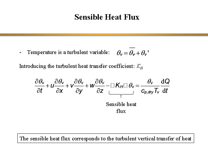
Sensible Heat Flux - Temperature is a turbulent variable: Zone KH Introducing the turbulent heat transfer coefficient: Sensible heat flux The sensible heat flux corresponds to the turbulent vertical transfer of heat

Latent Heat Flux The latent heat flux corresponds to the water vapor flux associated with evapotranspiration of vegetation and evaporation of water from surfaces. Zone This vertical transport of water vapor from the Earth’s surface to the atmosphere results from the heat added to the surface by solar radiation. When the water vapor condenses later in the atmosphere (leading to cloud formation), the condensation process leads to heat production. Therefore, the water vapor flux from the surface to the atmosphere corresponds to a hidden heat flux (from the latin “latens”, which means hidden).

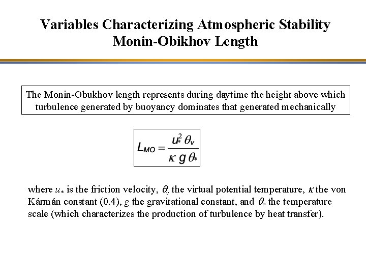
Variables Characterizing Atmospheric Stability Monin-Obikhov Length The Monin-Obukhov length represents during daytime the height above which turbulence generated by buoyancy dominates that generated mechanically Zone where u* is the friction velocity, qv the virtual potential temperature, k the von Kármán constant (0. 4), g the gravitational constant, and q* the temperature scale (which characterizes the production of turbulence by heat transfer).

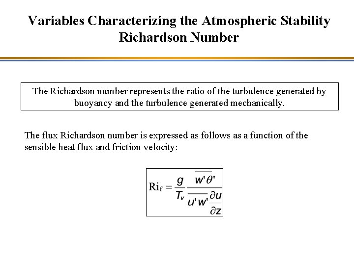
Variables Characterizing the Atmospheric Stability Richardson Number The Richardson number represents the ratio of the turbulence generated by buoyancy and the turbulence generated mechanically. Zone The flux Richardson number is expressed as follows as a function of the sensible heat flux and friction velocity:

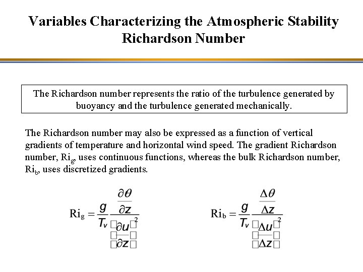
Variables Characterizing the Atmospheric Stability Richardson Number The Richardson number represents the ratio of the turbulence generated by buoyancy and the turbulence generated mechanically. Zone The Richardson number may also be expressed as a function of vertical gradients of temperature and horizontal wind speed. The gradient Richardson number, Rig, uses continuous functions, whereas the bulk Richardson number, Rib, uses discretized gradients.

Some Local-Scale Meteorological Phenomena - Land-sea breeze - Mountain-valley winds Zone - Urban heat island These phenomena affect the transport and dispersion of air pollutants.

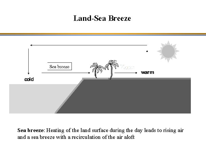
Land-Sea Breeze Sea breeze: Heating of the land surface during the day leads to rising air and a sea breeze with a recirculation of the air aloft

Land-Sea Breeze Land breeze: Cooling of the land surface at night leads to subsiding air and a land breeze with a recirculation of the air aloft

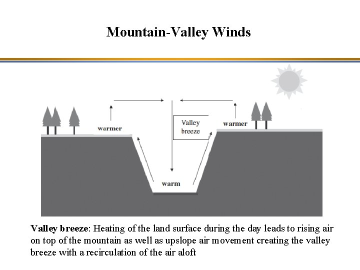
Mountain-Valley Winds Valley breeze: Heating of the land surface during the day leads to rising air on top of the mountain as well as upslope air movement creating the valley breeze with a recirculation of the air aloft

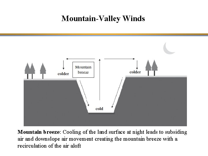
Mountain-Valley Winds Mountain breeze: Cooling of the land surface at night leads to subsiding air and downslope air movement creating the mountain breeze with a recirculation of the air aloft

Urban Heat Island Urban heat island: Urban areas are warmer than surrounding rural areas because of lower albedo (more short-wave solar radiation is stored during the day), heat production (heating, traffic…), and less evapotranspiration (less vegetation).

Air Pollution Episodes Air pollution episodes are favored by anticyclonic (high pressure) conditions with low wind speeds, which limit the advection and dispersion of pollutants. The clear skies associated with high pressure systems favor atmospheric chemistry and the formation of secondary pollutants, such as ozone and fine particulate matter (PM). The presence of a strong temperature inversion at night and/or in winter limits the vertical dispersion of pollutants emitted or formed within the mixing layer. Thus, it is conducive to high concentrations of primary pollutants emitted near the surface (e. g. , from traffic and residential heating).