AFD EFD CFD Fluid Mechanics Fluids are essential

AFD

EFD

CFD

Fluid Mechanics • Fluids are essential to life • Human body 70% water – Earth’s surface is 2/3 water – Atmosphere (troposphere) extends 17 km above the earth’s surface • History shaped by fluid mechanics – Geomorphology – Human migration and civilization – Modern scientific and mathematical theories and methods – Warfare • Affects every part of our lives

History Faces of Fluid Mechanics Archimedes (C. 287 -212 BC) Newton (1642 -1727) Leibniz (1646 -1716) Bernoulli (16671748)

Euler (17071783) Navier (1785 -1836) Stokes (18191903) Reynolds (1842 -1912)

Prandtl (1875 -1953) Taylor (1886 -1975)

Significance • Fluids omnipresent – Weather & climate – Vehicles: automobiles, trains, ships, and planes, etc. – Environment – Physiology and medicine – Sports & recreation – Many other examples!

Weather & Climate Tornadoes Thunderstorm

Global Climate Hurricanes

High-speed rail Submarines

Environment Air pollution River hydraulics

Physiology and Medicine Blood pump Ventricular assist device

Sports & Recreation Water sports Cycling

Offshore racing Auto racing

Surfing

Analytical Fluid Dynamics • The theory of mathematical physics problem formulation • Control volume & differential analysis • Exact solutions only exist for simple geometry and conditions • Approximate solutions for practical applications – Linear – Empirical relations using EFD data

Analytical Fluid Dynamics • Lecture Part of Fluid Class • Definition and fluids properties • Fluid statics • Fluids in motion • Continuity, momentum, and energy principles • Dimensional analysis and similitude • Surface resistance • Flow in conduits • Drag and lift

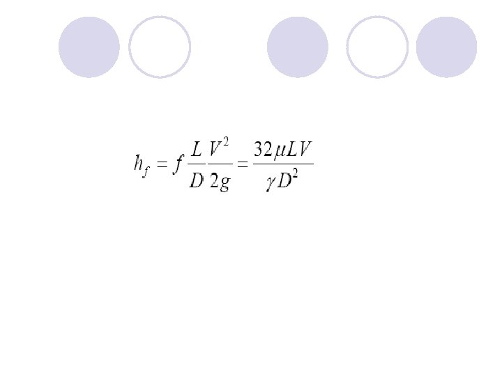
Analytical Fluid Dynamics • Example: laminar pipe flow Assumptions: Fully developed, Low Approach: Simplify momentum equation, integrate, apply boundary conditions to determine integration constants and use energy equation to calculate head loss

Exact solution :

Friction factor: Head loss: Schematic

Analytical Fluid Dynamics • Example: turbulent flow in smooth pipe (Re>3000) Three layer concept (using dimensional analysis)

1. Laminar sub-layer (viscous shear dominates) 2. Overlap layer (viscous and turbulent shear important) (&=0. 41, B=5. 5) 3. Outer layer (turbulent shear dominates)

Assume log-law is valid across entire pipe: Integration for average velocity and using EFD data to adjust constants:

Analytical Fluid Dynamics • Example: turbulent flow in rough pipe Both laminar sublayer and overlap layer are affected by roughness Inner layer: Outer layer: unaffected Overlap layer:

Three regimes of flow depending on k+ 1. k+<5, hydraulically smooth (no effect of roughness) 2. 5 < k+< 70, transitional roughness (Re dependent) 3. k+> 70, fully rough (independent Re) For 3, using EFD data to adjust constants: Friction factor:

Analytical Fluid Dynamics • Example: Moody diagram for turbulent pipe flow Composite Log-Law for smooth and rough pipes is given by the Moody diagram:

Experimental Fluid Dynamics (EFD) Definition: Use of experimental methodology and procedures for solving fluids engineering systems, including full and model scales, large and table top facilities, measurement systems (instrumentation, data acquisition and data reduction), uncertainty analysis, and dimensional analysis and similarity.

EFD philosophy: • Decisions on conducting experiments are governed by the ability of the expected test outcome, to achieve the test objectives within allowable uncertainties. • Integration of UA into all test phases should be a key part of entire experimental program • test design • determination of error sources • estimation of uncertainty • documentation of the results

Purpose • Science & Technology: understand investigate a phenomenon/process, substantiate and validate a theory (hypothesis) • Research & Development: document a process/system, provide benchmark data (standard procedures, validations), calibrate instruments, equipment, and facilities • Industry: design optimization and analysis, provide data for direct use, product liability, and acceptance • Teaching: instruction/demonstration

Applications of EFD Application in science & technology Picture of Karman vortex shedding Application in research & development Tropic Wind Tunnel has the ability to create temperatures ranging from 0 to 165 degrees Fahrenheit and simulate rain

Applications of EFD (cont’d) Example of industrial application NASA's cryogenic wind tunnel simulates flight conditions for scale models--a critical tool in designing airplanes. Application in teaching Fluid dynamics laboratory

Full and model scale • Scales: model, and full-scale • Selection of the model scale: governed by similarity dimensional analysis and

Measurement systems • Instrumentation • Load cell to measure forces and moments • Pressure transducers • Pitot tubes • Hotwire anemometry • PIV, LDV • Data acquisition • Serial port devices • Desktop PC’s • Plug-in data acquisition boards • Data Acquisition software - Labview • Data analysis and data reduction • Data reduction equations • Spectral analysis

Instrumentation Load cell Hotwire Pitot tube 3 D - PIV

Data acquisition system Hardware Software - Labview

Dimensional analysis • Definition : Dimensional analysis is a process of formulating fluid mechanics problems in terms of non-dimensional variables and parameters. • Why is it used : • Reduction in variables ( If F(A 1, A 2, … , An) = 0, then f(Π 1, Π 2, … Πr < n)= 0, here, F = functional form, Ai = dimensional variables, Πj = non dimensional parameters, m = number of important dimensions, n = number of dimensional variables, r= n – m ). Thereby the number of experiments required to determine f vs. F is reduced. • Helps in understanding physics • Useful in data analysis and modeling • Enables scaling of different physical dimensions and fluid properties

Example Drag = f(V, L, r, m, c, t, e, T, etc. ) From dimensional analysis, Vortex shedding behind cylinder

Examples of dimensionless quantities : Reynolds number, Froude Number, Strouhal number, Euler number, etc.

Similarity and model testing • Definition : Flow conditions for a model test are completely similar if all relevant dimensionless parameters have the same corresponding values for model and prototype. • Πi model = Πi prototype i = 1 • Enables extrapolation from model to full scale • However, complete similarity usually not possible. Therefore, often it is necessary to use Re, or Fr, or Ma scaling, i. e. , select most important Π and accommodate others as best possible.

• Types of similarity: • Geometric Similarity : all body dimensions in all three coordinates have the same linear-scale rations. • Kinematic Similarity : homologous (same relative position) particles lie at homologous points at homologous times. • Dynamic Similarity : in addition to the requirements for kinematic similarity the model and prototype forces must be in a constant ratio.

EFD process • “EFD process” is the steps to set up an experiment and take data

EFD – “hands on” experience Lab 1: Measurement of density and kinematic viscosity of a fluid Lab 2: Measurement of flow rate, friction factor and velocity profiles in smooth and rough pipes. Lab 3: Measurement of surface pressure Distribution, lift and drag coefficient for an airfoil

Computational Fluid Dynamics • CFD is use of computational methods for solving fluid engineering systems, including modeling (mathematical & Physics) and numerical methods (solvers, finite differences, and grid generations, etc. ). • Rapid growth in CFD technology since advent of computer ENIAC 1, 1946 IBM Work. Station

Purpose • The objective of CFD is to model the continuous fluids with Partial Differential Equations (PDEs) and discretize PDEs into an algebra problem, solve it, validate it and achieve simulation based design instead of “build & test” • Simulation of physical fluid phenomena that are difficult to be measured by experiments: scale simulations (full-scale ships, airplanes), hazards (explosions, radiations, pollution), physics (weather prediction, planetary boundary layer, stellar evolution).

Modeling • Mathematical physics problem formulation of fluid engineering system • Governing equations: Navier-Stokes equations (momentum), continuity equation, pressure Poisson equation, energy equation, ideal gas law, combustions (chemical reaction equation), multi-phase flows (e. g. Rayleigh equation), and turbulent models (RANS, LES, DES). • Coordinates: Cartesian, cylindrical and spherical coordinates result in different form of governing equation • Initial conditions (initial guess of the solution) and Boundary Conditions (no-slip wall, free-surface, zero-gradient, symmetry, velocity/pressure inlet/outlet) • Flow conditions: Geometry approximation, domain, Reynolds Number, and Mach Number, etc.

Modeling (examples) Free surface animation for ship in regular waves Developing flame surface (Bell et al. , 2001) Evolution of a 2 D mixing layer laden with particles of Stokes Number 0. 3 with respect to the vortex time scale (C. Narayanan)

Modeling (examples, cont’d) LES of a turbulent jet. Back wall shows a slice of the dissipation rate and the bottom wall shows a carpet plot of the mixture fraction in a slice through the jet centerline, Re=21, 000 (D. Glaze). DES, Re=105, Isosurface of Q criterion (0. 4) for turbulent flow around NACA 12 with angle of attack 60 degrees

Numerical methods • Finite difference methods: using numerical scheme to approximate the exact derivatives in the PDEs • Finite volume methods • Grid generation: conformal mapping, algebraic methods and differential equation methods • Grid types: structured, unstrctured

• Solvers: direct methods (Cramer’s rule, Gauss elimination, LU decomposition) and iterative methods (Jacobi, Gauss. Seidel, SOR) Slice of 3 D mesh of a fighter aircraft

CFD process

Commercial software • CFD software 1. FLUENT: http: //www. fluent. com 2. FLOWLAB: http: //www. flowlab. fluent. com 3. CFDRC: http: //www. cfdrc. com 4. STAR-CD: http: //www. cd-adapco. com 5. CFX/AEA: http: //www. software. aeat. com/cfx • Grid Generation software 1. Gridgen: http: //www. pointwise. com 2. Grid. Pro: http: //www. gridpro. com • Visualization software 1. Tecplot: http: //www. amtec. com 2. Fieldview: http: //www. ilight. com