8 Recurrent associative networks and episodic memory Fundamentals

8. Recurrent associative networks and episodic memory Fundamentals of Computational Neuroscience, T. P. Trappenberg, 2010. Lecture Notes on Brain and Computation Byoung-Tak Zhang Biointelligence Laboratory School of Computer Science and Engineering Graduate Programs in Cognitive Science, Brain Science and Bioinformatics Brain-Mind-Behavior Concentration Program Seoul National University E-mail: btzhang@bi. snu. ac. kr This material is available online at http: //bi. snu. ac. kr/ 1

Outline 8. 1 The auto-associative network and the hippocampus 8. 2 Point-attractor neural networks 8. 3 Sparse attractor networks and correlated patterns 8. 4 Chaotic networks: a dynamic systems view (C) 2010 SNU CSE Biointelligence Lab, http: //bi. snu. ac. kr 2

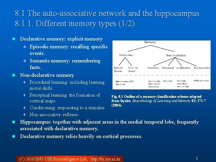
8. 1 The auto-associative network and the hippocampus 8. 1. 1. Different memory types (1/2) Declarative memory: explicit memory ¨ Episodic memory: recalling specific events. ¨ Semantic memory: remembering facts. l Non-declarative memory l ¨ Procedural learning: including learning motor skills. ¨ Perceptual learning: the formation of cortical maps. ¨ Conditioning: responding to a stimulus. ¨ Non-associative: reflexes. Fig. 8. 1 Outline of a memory classification scheme adapted from Squire, Neurobiology of Learning and Memory 82: 171 -7 (2004). Hippocampus: together with adjacent areas in the medial temporal lobe, frequently associated with declarative memory. l Declarative memory relies heavily on cortical processes. l (C) 2010 SNU CSE Biointelligence Lab, http: //bi. snu. ac. kr 3

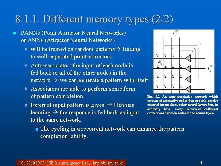
8. 1. 1. Different memory types (2/2) l PANNs (Point Attractor Neural Networks) or ANNs (Attractor Neural Networks) ¨ will be trained on random patterns leading to well-separated point-attractors. ¨ Auto-associator: the input of each node is fed back to all of the other nodes in the network we can generate a pattern with itself. ¨ Associators are able to perform some form Fig. 8. 2 An auto-associative network which of pattern completion. consists of associative nodes that not only receive external inputs from other neural layers but, in ¨ External input pattern is given Hebbian addition, have many recurrent collateral learning the response is fed back as input connections between nodes in the neural layer. to the same network. < The cycling in a recurrent network can enhance the pattern completion ability. (C) 2010 SNU CSE Biointelligence Lab, http: //bi. snu. ac. kr 4

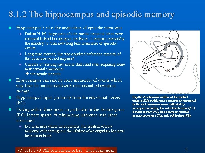
8. 1. 2 The hippocampus and episodic memory l Hippocampus’s role: the acquisition of episodic memories. ¨ Patient H. M. : large parts of both medial temporal lobes were removed to treat his epileptic condition amnesia marked by the inability to form new long-term memories of episodic events. ¨ Long-term memory that was acquired before the removal of this structure was not impaired. ¨ Capable of learning new motor skills and even acquiring some new semantic memories retrograde amnesia. l l l Hippocampus can rapidly store memories of events which may later be consolidated with neocortical information storage. Hippocampus input: primarily from the entorhinal cortex (EC). Coding within these areas, in particular in the dentate gyrus (DG) is very sparse minimizing inference with other memories. Fig. 8. 3 A schematic outline of the medial temporal lobe with some connections mentioned in the text. Some areas are indicated by acronyms including the entorhinal cortex (EC), dentate gyrus (DG), hippocampus subfield cornus ammonis (CA), and subiculum (SB). ¨ DG is an area where neurogenesis, the creation of new neuronal cells throughout the lifetime of an organism has now been established. (C) 2010 SNU CSE Biointelligence Lab, http: //bi. snu. ac. kr 5

8. 1. 3 Learning and retrieval phase l A difficulty in combining associative Hebbian mechanisms with recurrences in the networks ¨ Associative learning: relating presynaptic activity to postsynaptic activity imposed by an unconditional stimulus. ¨ The Recurrent network: drives this postsynaptic activity rapidly away from the activity pattern which one wants to imprint if the dynamic of the recurrent network is dominant. Solution: two phases operation of training and retrieval. ¨ In the hippocampus < Mossy fibres from granule cells in the DG provide strong inputs to CA 3 firing patterns could be dominated by this pathway during a learning phase. – The perforant pathway could stimulate the CA 4 neurons in the retrieval phase, where the CA 3 collateral and CA 3 -CA 1 projections could help to complete patterns from partial inputs. < Chemical agents such as acetylcholine (ACh) and noadrenaline could modulate learning and thereby enable the switching between a retrieval and learning phase. (C) 2010 SNU CSE Biointelligence Lab, http: //bi. snu. ac. kr 6

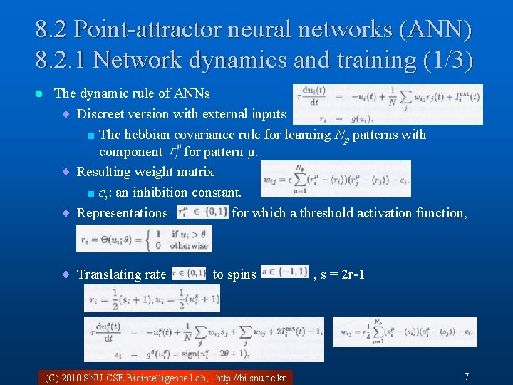
8. 2 Point-attractor neural networks (ANN) 8. 2. 1 Network dynamics and training (1/3) l The dynamic rule of ANNs ¨ Discreet version with external inputs < The hebbian covariance rule for learning Np patterns with component for pattern μ. ¨ Resulting weight matrix < ci: an inhibition constant. ¨ Representations for which a threshold activation function, ¨ Translating rate to spins (C) 2010 SNU CSE Biointelligence Lab, http: //bi. snu. ac. kr , s = 2 r-1 7

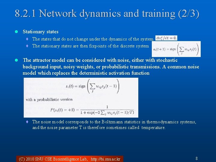
8. 2. 1 Network dynamics and training (2/3) l Stationary states ¨ The states that do not change under the dynamics of the system ¨ The stationary states are then fixpoints of the discrete system l The attractor model can be considered with noise, either with stochastic background input, noisy weights, or probabilistic transmissions. A common noise model which replaces the deterministic activation function ¨ The noise model corresponds to the Boltzmann statistics in thermodynamics systems, and the noise parameter T is therefore sometimes called temperature. (C) 2010 SNU CSE Biointelligence Lab, http: //bi. snu. ac. kr 8

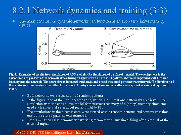
8. 2. 1 Network dynamics and training (3/3) l The main conclusion: dynamic networks can function as an auto-associative memory device. Fig. 8. 4 Examples of results from simulation of ANN models. (A) Simulation of the fixpoint model. The overlap here is the normalized dot product of the network states during an update with all of the 10 patterns that were imprinted with Hebbian learning into the network. The network was initialized randomly, and one of the stored patterns was retrieved. (B) Simulation of the continuous time version of an attractor network. A noisy version of one stored pattern was applied as external input until t=10τ. ¨ Both networks were trained on 10 random patterns. ¨ In the figure, one of the lines becomes one, which shows that one pattern was retrieved. The simulation with the continuous model demonstrates recovery of a (noisy) memory since one used such a noisy state as input pattern until t=10τ. ¨ The simulations in the discrete case were started with a random patterns and demonstrate that one of the stored patterns was retrieved. ¨ Both simulations also demonstrate working memory with sustained firing after removal of the external input. (C) 2010 SNU CSE Biointelligence Lab, http: //bi. snu. ac. kr 9

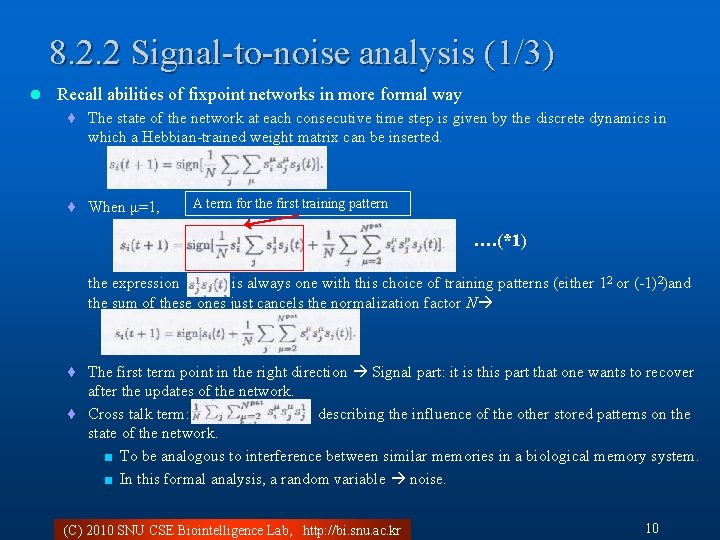
8. 2. 2 Signal-to-noise analysis (1/3) l Recall abilities of fixpoint networks in more formal way ¨ The state of the network at each consecutive time step is given by the discrete dynamics in which a Hebbian-trained weight matrix can be inserted. ¨ When μ=1, A term for the first training pattern …. (*1) the expression is always one with this choice of training patterns (either 12 or (-1)2)and the sum of these ones just cancels the normalization factor N ¨ The first term point in the right direction Signal part: it is this part that one wants to recover after the updates of the network. ¨ Cross talk term: describing the influence of the other stored patterns on the state of the network. < To be analogous to interference between similar memories in a biological memory system. < In this formal analysis, a random variable noise. (C) 2010 SNU CSE Biointelligence Lab, http: //bi. snu. ac. kr 10

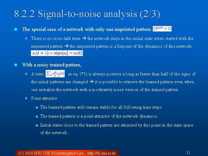
8. 2. 2 Signal-to-noise analysis (2/3) l The special case of a network with only one imprinted pattern ¨ There is no cross-talk term the network stays in the initial state when started with the imprinted pattern is a fixpoint of the dynamics of this network. l With a noisy trained pattern, ¨ A term in eq. (*1) is always positive a long as fewer than half of the signs of the initial patterns are changed it is possible to retrieve the learned pattern even when one initialize the network with a moderately noisy version of the trained pattern. ¨ Point attractor < The learned pattern will remain stable for all following time steps. < The trained pattern is a point attractor of the network dynamics. < Initial states close to the trained pattern are attracted by this point in the state space of the network. (C) 2010 SNU CSE Biointelligence Lab, http: //bi. snu. ac. kr 11

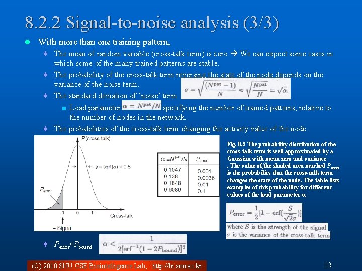
8. 2. 2 Signal-to-noise analysis (3/3) l With more than one training pattern, ¨ The mean of random variable (cross-talk term) is zero We can expect some cases in which some of the many trained patterns are stable. ¨ The probability of the cross-talk term reversing the state of the node depends on the variance of the noise term. ¨ The standard deviation of ‘noise’ term < Load parameter specifying the number of trained patterns, relative to the number of nodes in the network. ¨ The probabilities of the cross-talk term changing the activity value of the node. Fig. 8. 5 The probability distribution of the cross-talk term is well approximated by a Gaussian with mean zero and variance. The value of the shaded area marked Perror is the probability that the cross-talk term changes the state of the node. The table lists examples of this probability for different values of the load parameter α. ¨ Perror<Pbound (C) 2010 SNU CSE Biointelligence Lab, http: //bi. snu. ac. kr 12

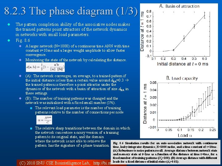
8. 2. 3 The phase diagram (1/3) l l The pattern completion ability of the associative nodes makes the trained patterns point attractors of the network dynamics in networks with small load parameters. Fig. 8. 6 ¨ A larger network (N=1000) of a continuous time ANN with time constant τ=10 ms and a larger weight amplitude to allow faster convergence. ¨ Monitoring the state of the network by calculating the distance. ¨ (A): The network converges, on average, to a trained pattern if the initial distance is less than a certain value around d. BA≈0. 3 the trained pattern is therefore a point attractor under the dynamics of the network with a basin of attraction of size d. BA in these settings. ¨ (B): The number of training patterns was changed and the network was initialized with a fixed small number (1%). < The relevant load parameter is the number of training patterns relative to the number of connections per node < The relative sharp transitions between the domain in which the network can restore a noisy version of a training pattern to its original state, and the domain where the network is not able to retrieve the Fig. 8. 6 Simulation results for an auto-associative network with continuous pattern has the signature of a phase transition. time, leaky-integrator dynamics, N=1000 nodes, and a time constant of τ=10 ms. (A) Robustness to noise pattern recall. Average distance between network state and memory state at t=1 ms as a function of the distance at time t=0 ms, for a fixed number of training patterns (Np=100). (B) Average distance with different loads for a fixed distance of initial states (d 0=0. 01). 13 (C) 2010 SNU CSE Biointelligence Lab, http: //bi. snu. ac. kr

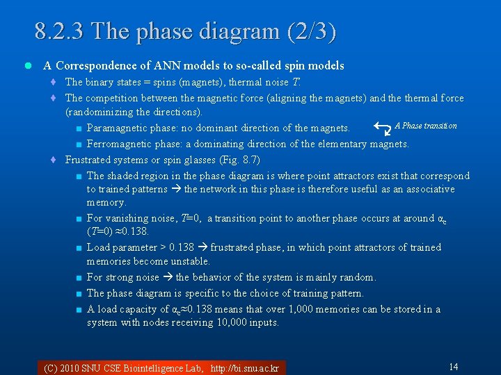
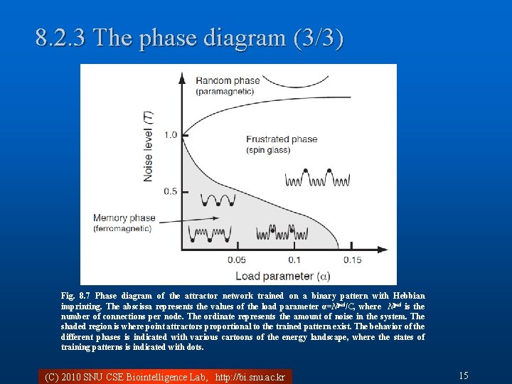
8. 2. 3 The phase diagram (2/3) l A Correspondence of ANN models to so-called spin models ¨ The binary states = spins (magnets), thermal noise T. ¨ The competition between the magnetic force (aligning the magnets) and thermal force (randominizing the directions). A Phase transition < Paramagnetic phase: no dominant direction of the magnets. < Ferromagnetic phase: a dominating direction of the elementary magnets. ¨ Frustrated systems or spin glasses (Fig. 8. 7) < The shaded region in the phase diagram is where point attractors exist that correspond to trained patterns the network in this phase is therefore useful as an associative memory. < For vanishing noise, T=0, a transition point to another phase occurs at around αc (T=0) ≈0. 138. < Load parameter > 0. 138 frustrated phase, in which point attractors of trained memories become unstable. < For strong noise the behavior of the system is mainly random. < The phase diagram is specific to the choice of training pattern. < A load capacity of αc≈0. 138 means that over 1, 000 memories can be stored in a system with nodes receiving 10, 000 inputs. (C) 2010 SNU CSE Biointelligence Lab, http: //bi. snu. ac. kr 14

8. 2. 3 The phase diagram (3/3) Fig. 8. 7 Phase diagram of the attractor network trained on a binary pattern with Hebbian imprinting. The abscissa represents the values of the load parameter α=Npat/C, where Npat is the number of connections per node. The ordinate represents the amount of noise in the system. The shaded region is where point attractors proportional to the trained pattern exist. The behavior of the different phases is indicated with various cartoons of the energy landscape, where the states of training patterns is indicated with dots. (C) 2010 SNU CSE Biointelligence Lab, http: //bi. snu. ac. kr 15

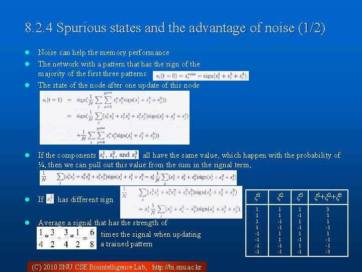
8. 2. 4 Spurious states and the advantage of noise (1/2) l l l Noise can help the memory performance The network with a pattern that has the sign of the majority of the first three patterns: The state of the node after one update of this node l If the components all have the same value, which happen with the probability of ¼, then we can pull out this value from the sum in the signal term, l If l has different sign Average a signal that has the strength of times the signal when updating a trained pattern (C) 2010 SNU CSE Biointelligence Lab, http: //bi. snu. ac. kr ξ 1 ξ 2 ξ 3 ξ 1+ξ 2+ξ 3 1 1 -1 -1 1 -1 3 1 1 -1 -1 -3

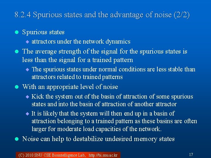
8. 2. 4 Spurious states and the advantage of noise (2/2) l Spurious states ¨ attractors under the network dynamics l The average strength of the signal for the spurious states is less than the signal for a trained pattern ¨ The spurious states under normal conditions are less stable than attractors related to trained patterns l With an appropriate level of noise ¨ Kick the system out of the basin of attraction of some spurious states and into the basin of attraction of another attractor ¨ It is likely that the system will then end up in a basin of attraction belonging to a trained pattern as these basins are often larger for moderate load capacities of the network. l Noise can help to destabilize undesired memory states (C) 2010 SNU CSE Biointelligence Lab, http: //bi. snu. ac. kr 17

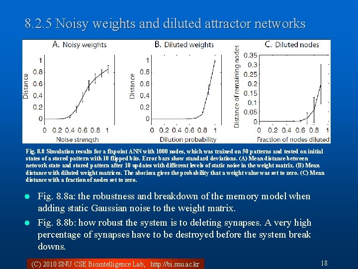
8. 2. 5 Noisy weights and diluted attractor networks Fig. 8. 8 Simulation results for a fixpoint ANN with 1000 nodes, which was trained on 50 patterns and tested on initial states of a stored pattern with 10 flipped bits. Error bars show standard deviations. (A) Mean distance between network state and stored pattern after 10 updates with different levels of static noise in the weight matrix. (B) Mean distance with diluted weight matrices. The abscissa gives the probability that a weight value was set to zero. (C) Mean distance with a fraction of nodes set to zero. Fig. 8. 8 a: the robustness and breakdown of the memory model when adding static Gaussian noise to the weight matrix. l Fig. 8. 8 b: how robust the system is to deleting synapses. A very high percentage of synapses have to be destroyed before the system break downs. l (C) 2010 SNU CSE Biointelligence Lab, http: //bi. snu. ac. kr 18

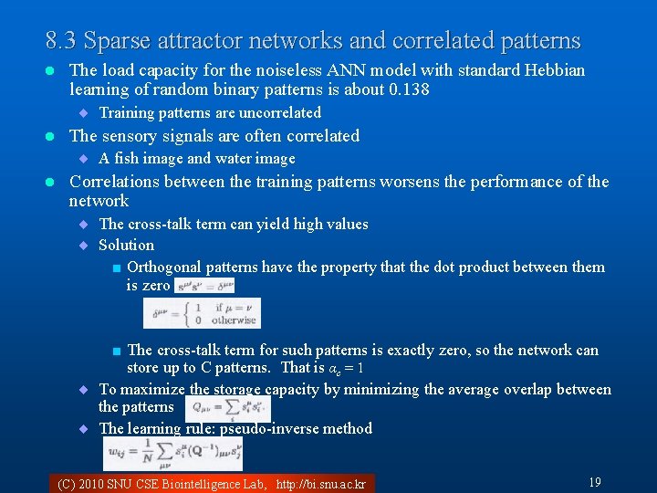
8. 3 Sparse attractor networks and correlated patterns l The load capacity for the noiseless ANN model with standard Hebbian learning of random binary patterns is about 0. 138 ¨ Training patterns are uncorrelated l The sensory signals are often correlated ¨ A fish image and water image l Correlations between the training patterns worsens the performance of the network ¨ The cross-talk term can yield high values ¨ Solution < Orthogonal patterns have the property that the dot product between them is zero < The cross-talk term for such patterns is exactly zero, so the network can store up to C patterns. That is αc = 1 ¨ To maximize the storage capacity by minimizing the average overlap between the patterns ¨ The learning rule: pseudo-inverse method (C) 2010 SNU CSE Biointelligence Lab, http: //bi. snu. ac. kr 19

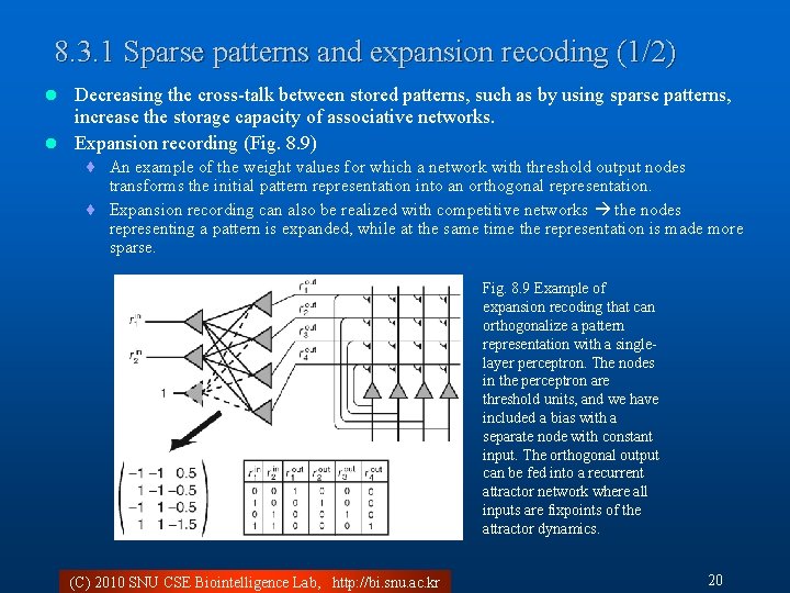
8. 3. 1 Sparse patterns and expansion recoding (1/2) Decreasing the cross-talk between stored patterns, such as by using sparse patterns, increase the storage capacity of associative networks. l Expansion recording (Fig. 8. 9) l ¨ An example of the weight values for which a network with threshold output nodes transforms the initial pattern representation into an orthogonal representation. ¨ Expansion recording can also be realized with competitive networks the nodes representing a pattern is expanded, while at the same time the representation is made more sparse. Fig. 8. 9 Example of expansion recoding that can orthogonalize a pattern representation with a singlelayer perceptron. The nodes in the perceptron are threshold units, and we have included a bias with a separate node with constant input. The orthogonal output can be fed into a recurrent attractor network where all inputs are fixpoints of the attractor dynamics. (C) 2010 SNU CSE Biointelligence Lab, http: //bi. snu. ac. kr 20

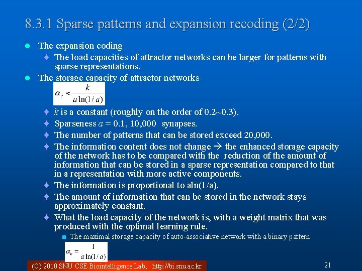
8. 3. 1 Sparse patterns and expansion recoding (2/2) The expansion coding ¨ The load capacities of attractor networks can be larger for patterns with sparse representations. l The storage capacity of attractor networks l ¨ ¨ k is a constant (roughly on the order of 0. 2~0. 3). Sparseness a = 0. 1, 10, 000 synapses. The number of patterns that can be stored exceed 20, 000. The information content does not change the enhanced storage capacity of the network has to be compared with the reduction of the amount of information that can be stored in a sparse representation compared to that in a representation with more active components. ¨ The information is proportional to aln(1/a). ¨ The amount of information that can be stored in the network stays approximately constant. ¨ What the load capacity of the network is, with a weight matrix that was produced with the optimal learning rule. < The maximal storage capacity of auto-associative network with a binary pattern (C) 2010 SNU CSE Biointelligence Lab, http: //bi. snu. ac. kr 21

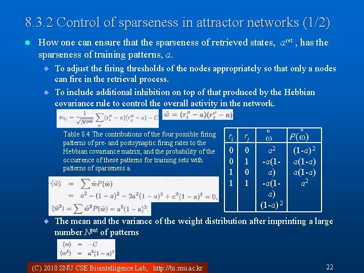
8. 3. 2 Control of sparseness in attractor networks (1/2) l How one can ensure that the sparseness of retrieved states, aret , has the sparseness of training patterns, a. ¨ To adjust the firing thresholds of the nodes appropriately so that only a nodes can fire in the retrieval process. ¨ To include additional inhibition on top of that produced by the Hebbian covariance rule to control the overall activity in the network. Table 8. 4 The contributions of the four possible firing patterns of pre- and postsynaptic firing rates to the Hebbian covariance matrix, and the probability of the occurrence of these patterns for training sets with patterns of sparseness a. ri rj 0 0 1 1 0 1 a 2 -a(1 a) (1 -a) 2 a(1 -a) a 2 ¨ The mean and the variance of the weight distribution after imprinting a large number Npat of patterns (C) 2010 SNU CSE Biointelligence Lab, http: //bi. snu. ac. kr 22

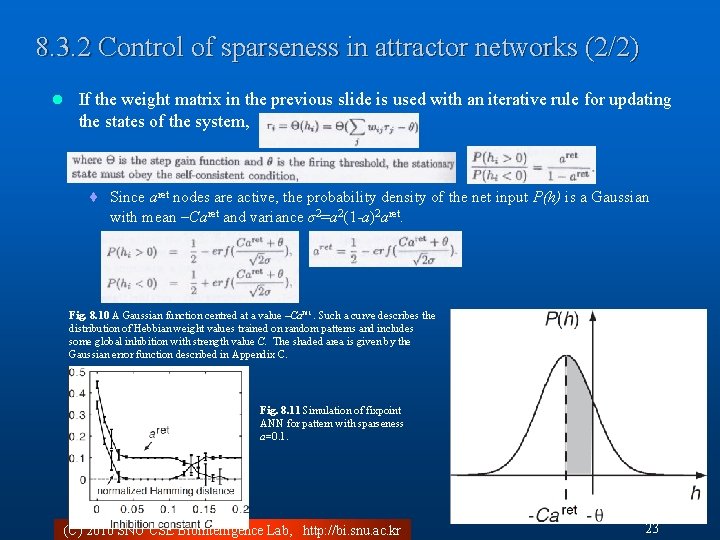
8. 3. 2 Control of sparseness in attractor networks (2/2) l If the weight matrix in the previous slide is used with an iterative rule for updating the states of the system, ¨ Since aret nodes are active, the probability density of the net input P(h) is a Gaussian with mean –Caret and variance σ2=a 2(1 -a)2 aret. Fig. 8. 10 A Gaussian function centred at a value –Caret. Such a curve describes the distribution of Hebbian weight values trained on random patterns and includes some global inhibition with strength value C. The shaded area is given by the Gaussian error function described in Appendix C. Fig. 8. 11 Simulation of fixpoint ANN for pattern with sparseness a=0. 1. (C) 2010 SNU CSE Biointelligence Lab, http: //bi. snu. ac. kr 23

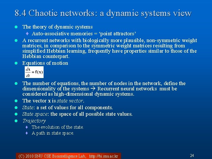
8. 4 Chaotic networks: a dynamic systems view The theory of dynamic systems ¨ Auto-associative memories = ‘point attractors’ l A recurrent networks with biologically more plausible, non-symmetric weight matrices, in comparison to the symmetric weight matrices resulting from simplified Hebbian learning, frequently have properties similar to those of the Hebbian counterpart. l Equations of motion l l l The number of equations, the number of nodes in the network, define the dimensionality of the systems Recurrent neural networks must be considered as high-dimensional dynamic systems. The vector x is state vector. State: a set of values for all components. State space: the space of all possible state values. Trajectory ¨ The evolution of the state. ¨ A path in state space. (C) 2010 SNU CSE Biointelligence Lab, http: //bi. snu. ac. kr 24

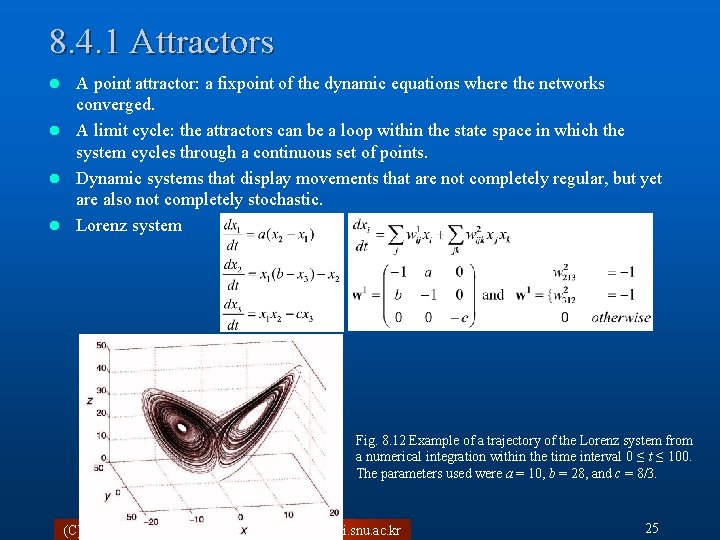
8. 4. 1 Attractors A point attractor: a fixpoint of the dynamic equations where the networks converged. l A limit cycle: the attractors can be a loop within the state space in which the system cycles through a continuous set of points. l Dynamic systems that display movements that are not completely regular, but yet are also not completely stochastic. l Lorenz system l Fig. 8. 12 Example of a trajectory of the Lorenz system from a numerical integration within the time interval 0 ≤ t ≤ 100. The parameters used were a = 10, b = 28, and c = 8/3. (C) 2010 SNU CSE Biointelligence Lab, http: //bi. snu. ac. kr 25

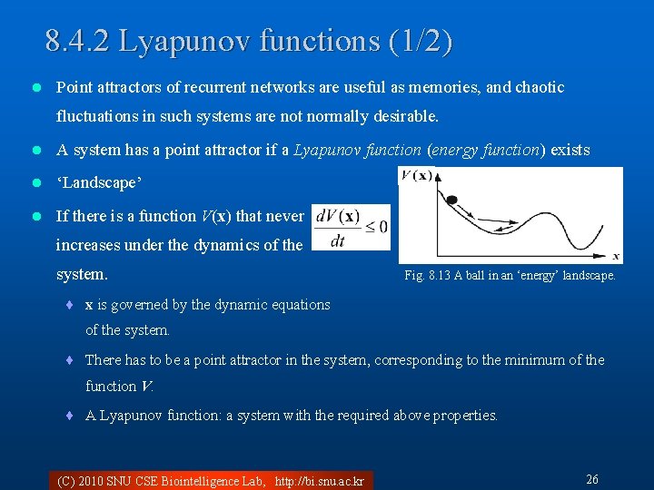
8. 4. 2 Lyapunov functions (1/2) l Point attractors of recurrent networks are useful as memories, and chaotic fluctuations in such systems are not normally desirable. l A system has a point attractor if a Lyapunov function (energy function) exists l ‘Landscape’ l If there is a function V(x) that never increases under the dynamics of the system. Fig. 8. 13 A ball in an ‘energy’ landscape. ¨ x is governed by the dynamic equations of the system. ¨ There has to be a point attractor in the system, corresponding to the minimum of the function V. ¨ A Lyapunov function: a system with the required above properties. (C) 2010 SNU CSE Biointelligence Lab, http: //bi. snu. ac. kr 26

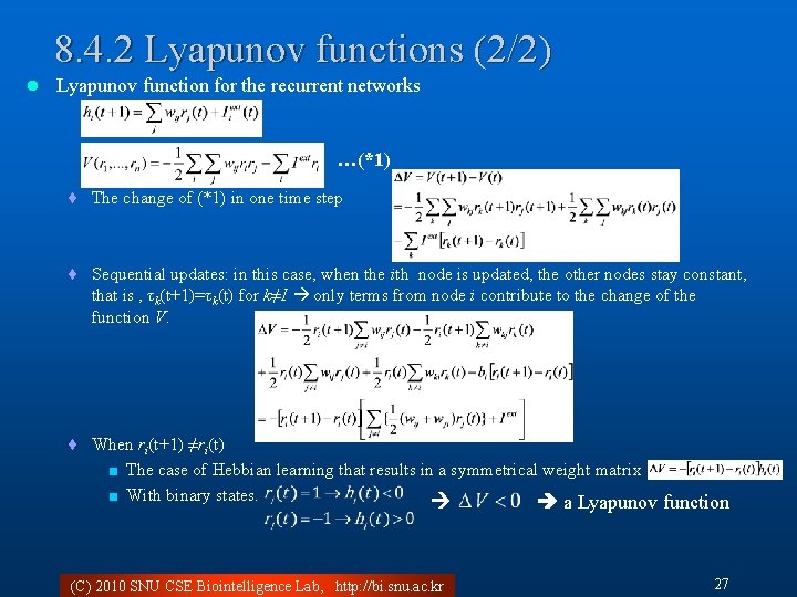
8. 4. 2 Lyapunov functions (2/2) l Lyapunov function for the recurrent networks …(*1) ¨ The change of (*1) in one time step ¨ Sequential updates: in this case, when the ith node is updated, the other nodes stay constant, that is , τk(t+1)=τk(t) for k≠I only terms from node i contribute to the change of the function V. ¨ When ri(t+1) ≠ri(t) < The case of Hebbian learning that results in a symmetrical weight matrix < With binary states. a Lyapunov function (C) 2010 SNU CSE Biointelligence Lab, http: //bi. snu. ac. kr 27

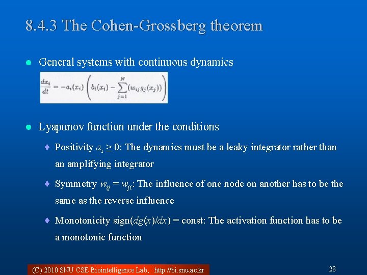
8. 4. 3 The Cohen-Grossberg theorem l General systems with continuous dynamics l Lyapunov function under the conditions ¨ Positivity ai ≥ 0: The dynamics must be a leaky integrator rather than an amplifying integrator ¨ Symmetry wij = wji: The influence of one node on another has to be the same as the reverse influence ¨ Monotonicity sign(dg(x)/dx) = const: The activation function has to be a monotonic function (C) 2010 SNU CSE Biointelligence Lab, http: //bi. snu. ac. kr 28

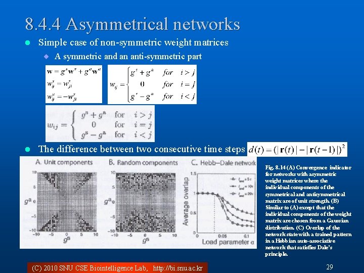
8. 4. 4 Asymmetrical networks l Simple case of non-symmetric weight matrices ¨ A symmetric and an anti-symmetric part l The difference between two consecutive time steps Fig. 8. 14 (A) Convergence indicator for networks with asymmetric weight matrices where the individual components of the symmetrical and antisymmetrical matrix are of unit strength. (B) Similar to (A) except that the individual components of the weight matrix are chosen from a Gaussian distribution. (C) Overlap of the network state with a trained pattern in a Hebbian auto-associative network that satisfies Dale’s principle. (C) 2010 SNU CSE Biointelligence Lab, http: //bi. snu. ac. kr 29

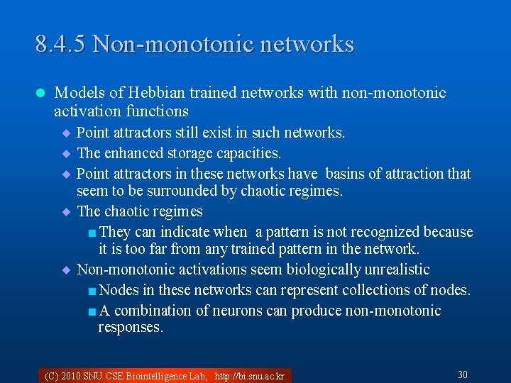
8. 4. 5 Non-monotonic networks l Models of Hebbian trained networks with non-monotonic activation functions ¨ Point attractors still exist in such networks. ¨ The enhanced storage capacities. ¨ Point attractors in these networks have basins of attraction that seem to be surrounded by chaotic regimes. ¨ The chaotic regimes < They can indicate when a pattern is not recognized because it is too far from any trained pattern in the network. ¨ Non-monotonic activations seem biologically unrealistic < Nodes in these networks can represent collections of nodes. < A combination of neurons can produce non-monotonic responses. (C) 2010 SNU CSE Biointelligence Lab, http: //bi. snu. ac. kr 30