Variational Approaches and Image Segmentation Lecture 6 Hossam

Variational Approaches and Image Segmentation Lecture #6 Hossam Abdelmunim 1 & Aly A. Farag 2 1 Computer & Systems Engineering Department, Ain Shams University, Cairo, Egypt 2 Electerical and Computer Engineering Department, University of Louisville, KY, USA ECE 643 – Fall 2010 1

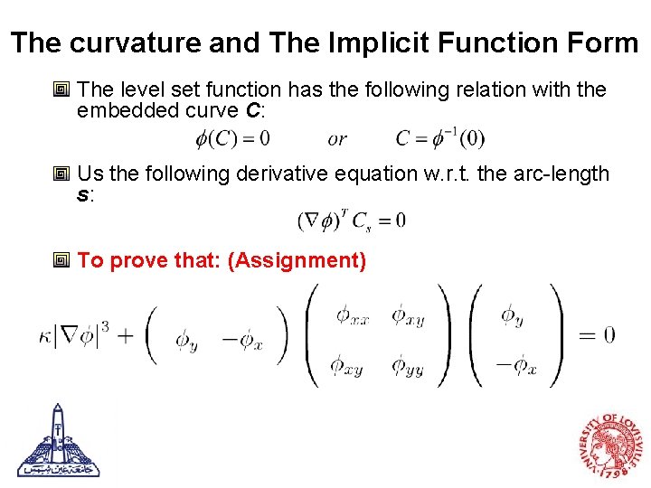
The curvature and The Implicit Function Form The level set function has the following relation with the embedded curve C: Us the following derivative equation w. r. t. the arc-length s: To prove that: (Assignment)

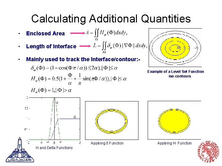
Calculating Additional Quantities • Enclosed Area • Length of Interface • Mainly used to track the Interface/contour: Example of a Level Set Function iso-contours Applying δ Function H and Delta Functions Applying H Function

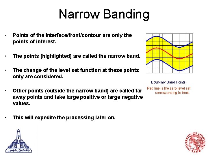
Narrow Banding • Points of the interface/front/contour are only the points of interest. • The points (highlighted) are called the narrow band. • The change of the level set function at these points only are considered. Boundary Band Points. • Other points (outside the narrow band) are called far away points and take large positive or large negative values. • This will expedite the processing later on. Red line is the zero level set corresponding to front.

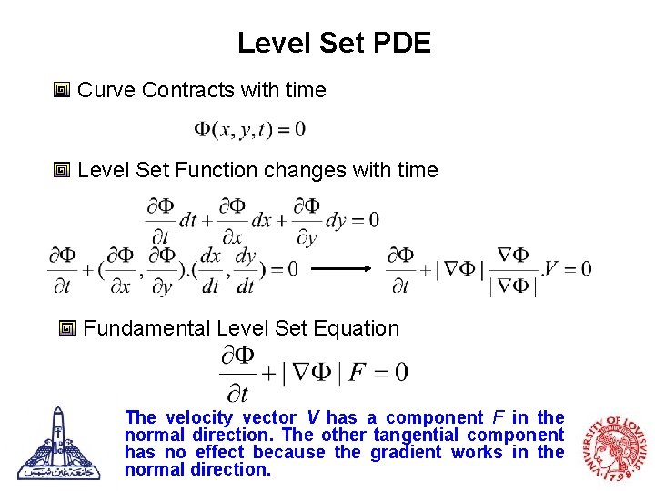
Level Set PDE Curve Contracts with time Level Set Function changes with time Fundamental Level Set Equation The velocity vector V has a component F in the normal direction. The other tangential component has no effect because the gradient works in the normal direction.

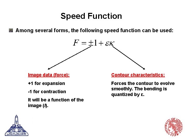
Speed Function Among several forms, the following speed function can be used: Image data (force): Contour characteristics: +1 for expansion Forces the contour to evolve smoothly. The bending is quantized by ε. -1 for contraction It will be a function of the image (I).

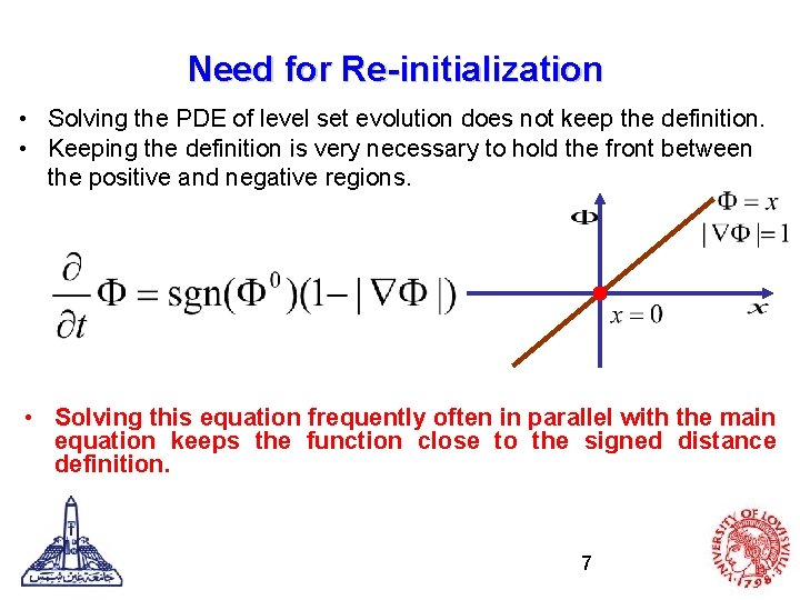
Need for Re-initialization • Solving the PDE of level set evolution does not keep the definition. • Keeping the definition is very necessary to hold the front between the positive and negative regions. • Solving this equation frequently often in parallel with the main equation keeps the function close to the signed distance definition. 7

Numerical Solution

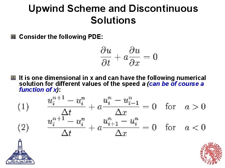
Upwind Scheme and Discontinuous Solutions Consider the following PDE: It is one dimensional in x and can have the following numerical solution for different values of the speed a (can be of course a function of x):

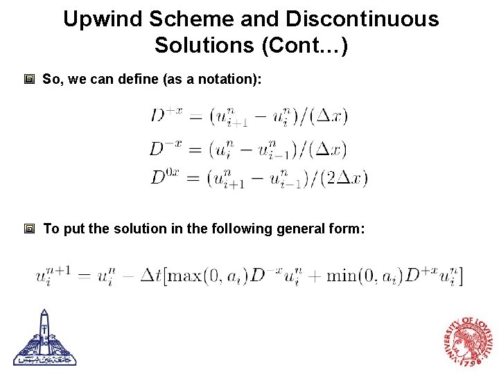
Upwind Scheme and Discontinuous Solutions (Cont…) So, we can define (as a notation): To put the solution in the following general form:

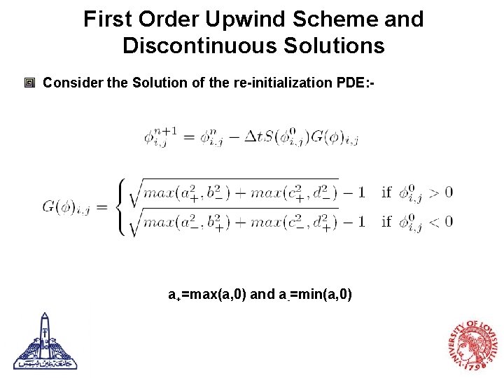
First Order Upwind Scheme and Discontinuous Solutions Consider the Solution of the re-initialization PDE: - a+=max(a, 0) and a-=min(a, 0)

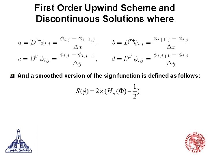
First Order Upwind Scheme and Discontinuous Solutions where And a smoothed version of the sign function is defined as follows:

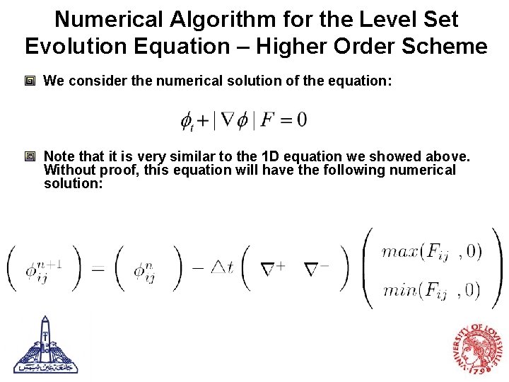
Numerical Algorithm for the Level Set Evolution Equation – Higher Order Scheme We consider the numerical solution of the equation: Note that it is very similar to the 1 D equation we showed above. Without proof, this equation will have the following numerical solution:

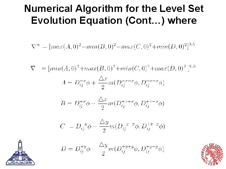
Numerical Algorithm for the Level Set Evolution Equation (Cont…) where

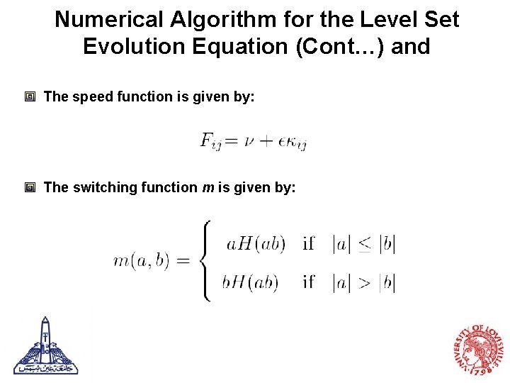
Numerical Algorithm for the Level Set Evolution Equation (Cont…) and The speed function is given by: The switching function m is given by:

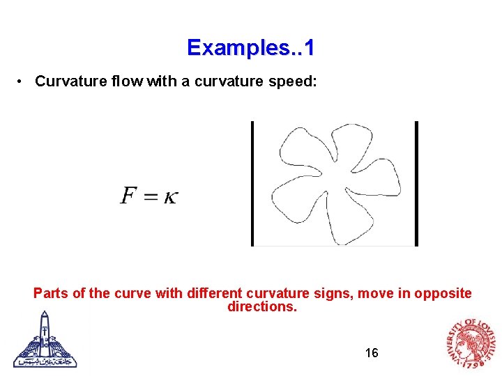
Examples. . 1 • Curvature flow with a curvature speed: Parts of the curve with different curvature signs, move in opposite directions. 16

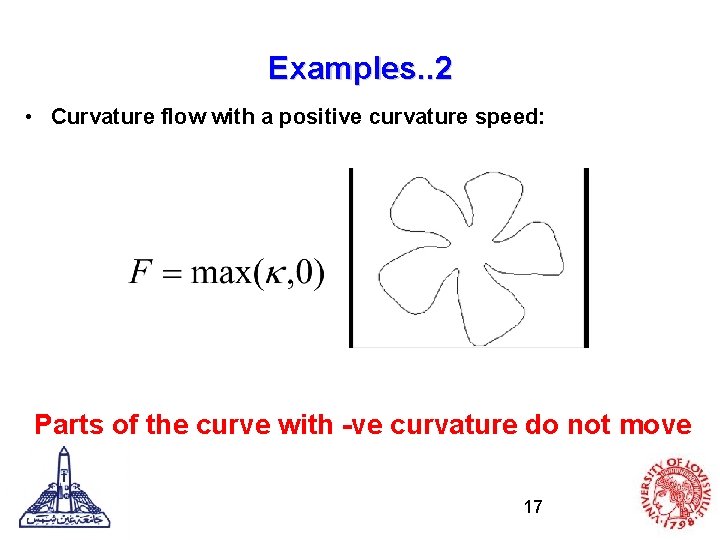
Examples. . 2 • Curvature flow with a positive curvature speed: Parts of the curve with -ve curvature do not move 17

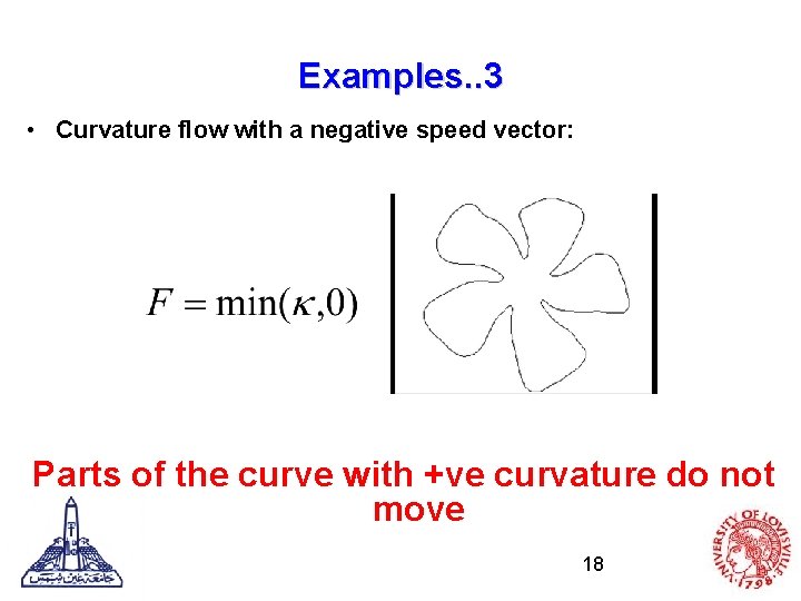
Examples. . 3 • Curvature flow with a negative speed vector: Parts of the curve with +ve curvature do not move 18