UNIT I Problem solving and Algorithmic Analysis Problem

UNIT- I Problem solving and Algorithmic Analysis Problem solving principles: Classification of problem, problem solving strategies, classification of time complexities (linear, logarithmic etc) problem subdivision { Divide and Conquer strategy}. Asymptotic notations, lower bound and upper bound: Best case, worst case, average case analysis, amortized analysis. Performance analysis of basic programming constructs. Recurrences: Formulation and solving recurrence equations using Master Theorem.

Recurrences • Recurrence: an equation that describes a function in terms of its value on smaller functions • The expression: is a recurrence.

Recurrence Examples

Solving Recurrences • Substitution method • Iteration method • Master method

The Master Theorem • Given: a divide and conquer algorithm – An algorithm that divides the problem of size n into a subproblems, each of size n/b – Let the cost of each stage (i. e. , the work to divide the problem + combine solved subproblems) be described by the function f(n) • Then, the Master Theorem gives us a cookbook for the algorithm’s running time:

 = a. T(n/b) + f(n) then")
The Master Theorem • if T(n) = a. T(n/b) + f(n) then

Divide and Conquer • Recursive in structure – Divide the problem into sub-problems that are similar to the original but smaller in size – Conquer the sub-problems by solving them recursively. If they are small enough, just solve them in a straightforward manner. – Combine the solutions to create a solution to the original problem Comp 122
 2. { 3. if small(P)")
Control abstraction of D&C Method 1. Algorithm DAnd. C(P) 2. { 3. if small(P) then return S(P); 4. else 5. { 6. divide P into smaller instances P 1, P 2… Pk, k>=1; 7. Apply DAnd. C to each of these sub problems; 8. return combine (DAnd. C(P 1), DAnd. C(P 2), . . , DAnd. C(Pk)); 9. } 10. }

• If size of P is n and the size of the k subproblems are n 1, n 2 …. . nk ten computing time of Dand. C is described by the recurrence relation • T(n)= g(n) n small T(n 1)+T(N 2)+…+T(nk)+f(n) otherwise • T(n) time for DAnd. C on any input of size n • g(n) time to compute the answer directly for small input • f(n) time for dividing P and combining the solution of subproblems.

• The complexity of many divide and conquer algorithm is given by recurrence of the form • T(n)= T(1) n small a. T(n/b)+f(n) otherwise • Where a and b are known constants. • We assume that T(1) is known and n is power of b that is n=bk

Example of Divide and Conquer • Binary Search • Merge Sort • Quick Sort

Binary Search • Let ai, 1 ≤ i ≤ n be a list of elements which are sorted in nondecreasing order. • Consider the problem of determining whether a given element x is present in the list. • If x is present, we are to determine a value j such that aj = x. • If x is not in the list then j is to be set to zero. • Divide-and-conquer suggests breaking up any instance I = (n, a 1, . . . , an. x) of this search problem into subinstances.
 //given an array A(i: l) of elements")
Binary Search Algorithm BINSRCH(a, i, l, x) //given an array A(i: l) of elements in nondecreasing order, 1 ≤ i ≤ l determine if x is present, and if so, set j such that x = a[j] else return 0 { if (l=i) then { if( x=a[i]) then return i; Else return 0; } Else { //reduce P into a smaller subproblem mid= �(i+l)/2 �; if (x=a[mid] )then return mid; Else if (x<a[mid]) then Return BINSRCH(a, i, mid-1, x); Else Return BINSRCH(a, i, mid+1, x); } }

Binary Search Ex. Binary search for 33. 6 0 lo 13 14 25 33 43 51 53 64 72 84 93 95 96 97 1 2 3 4 5 6 7 8 9 10 11 12 13 14 hi

Binary Search Ex. Binary search for 33. 6 0 lo 13 14 25 33 43 51 53 64 72 84 93 95 96 97 1 2 3 4 5 6 7 mid 8 9 10 11 12 13 14 hi

Binary Search Ex. Binary search for 33. 6 0 lo 13 14 25 33 43 51 53 64 72 84 93 95 96 97 1 2 3 4 5 6 hi 7 8 9 10 11 12 13 14

Binary Search Ex. Binary search for 33. 6 0 lo 13 14 25 33 43 51 53 64 72 84 93 95 96 97 1 2 3 mid 4 5 6 hi 7 8 9 10 11 12 13 14

Binary Search Ex. Binary search for 33. 6 0 13 14 25 33 43 51 53 64 72 84 93 95 96 97 1 2 3 4 lo 5 6 hi 7 8 9 10 11 12 13 14

Binary Search Ex. Binary search for 33. 6 0 13 14 25 33 43 51 53 64 72 84 93 95 96 97 1 2 3 4 5 6 lo mid hi 7 8 9 10 11 12 13 14

Binary Search Ex. Binary search for 33. 6 0 13 14 25 33 43 51 53 64 72 84 93 95 96 97 1 2 3 4 lo hi 5 6 7 8 9 10 11 12 13 14

Binary Search Ex. Binary search for 33. 6 0 13 14 25 33 43 51 53 64 72 84 93 95 96 97 1 2 3 4 lo hi mid 5 6 7 8 9 10 11 12 13 14

Binary Search Ex. Binary search for 33. 6 0 13 14 25 33 43 51 53 64 72 84 93 95 96 97 1 2 3 4 lo hi mid 5 6 7 8 9 10 11 12 13 14
 Best case Ө(log n) Average Case Ө(log n) Worst")
Successful Search Unsuccessful search Ө(1) Best case Ө(log n) Average Case Ө(log n) Worst Case Ө(log n)
 A(l), .")
Merge sort • Given a sequence of n. elements (also called keys) A(l), . . . , A(n) the general idea is to imagine them split into two sets A(1), . , A( n/2) and A( n/2 + 1), . . . , A(n). • Each set is individually sorted and the resulting sequences are merged to produce a single sorted sequence of n elements.
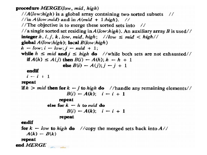
 //A(low : high) is a global array containing high - low")
Algorithm MERGESORT(low, high) //A(low : high) is a global array containing high - low + 1 ≥ 0 //values which represent the elements to be sorted. if low < high then mid �(low + high)/2 � //find where to split the set// call MERGESORT(low, mid) //sort one subset// call MERGESORT(mid + 1, high) //sort the other subset// call MERGE(low, mid, high) //combine the results/ Endif end MERGESORT
 of Merge Sort:")
• • • Analysis of Merge Sort Running time T(n) of Merge Sort: Divide: computing the middle takes (1) Conquer: solving 2 subproblems takes 2 T(n/2) Combine: merging n elements takes (n) Total: T(n) = (1) if n = 1 T(n) = 2 T(n/2) + (n) if n > 1 T(n) = (n log n) Comp 122

• If the time for the merging operation is proportional to n the computing time for mergesort is described by the recurrence relation • T(n) = a n = 1, a constant 2 T(n/2) + cn n > l, c constant • By using recurrence we got T(n) = O(n log 2 n)

Merging • The key to Merge Sort is merging two sorted lists into one, such that if you have two lists X (x 1 x 2 … xm) and Y(y 1 y 2 … yn) the resulting list is Z(z 1 z 2 … zm+n) • Example: L 1 = { 3 8 9 } L 2 = { 1 5 7 } merge(L 1, L 2) = { 1 3 5 7 8 9 }
 X: Result: 3 10 23 54 Y: 1 5 25 75")
Merging (cont. ) X: Result: 3 10 23 54 Y: 1 5 25 75
 X: Result: 3 10 1 23 54 Y: 5 25 75")
Merging (cont. ) X: Result: 3 10 1 23 54 Y: 5 25 75
 X: Result: 10 1 23 3 54 Y: 5 25 75")
Merging (cont. ) X: Result: 10 1 23 3 54 Y: 5 25 75
 X: Result: 10 1 23 3 54 5 Y: 25 75")
Merging (cont. ) X: Result: 10 1 23 3 54 5 Y: 25 75
 X: Result: 23 1 3 54 5 Y: 10 25 75")
Merging (cont. ) X: Result: 23 1 3 54 5 Y: 10 25 75
 X: Result: 54 1 3 5 Y: 10 25 23 75")
Merging (cont. ) X: Result: 54 1 3 5 Y: 10 25 23 75
 X: Result: 54 1 3 5 Y: 10 75 23 25")
Merging (cont. ) X: Result: 54 1 3 5 Y: 10 75 23 25
 X: Result: Y: 1 3 5 10 75 23 25 54")
Merging (cont. ) X: Result: Y: 1 3 5 10 75 23 25 54
 X: Result: Y: 1 3 5 10 23 25 54 75")
Merging (cont. ) X: Result: Y: 1 3 5 10 23 25 54 75

Merge Sort Example 99 6 86 15 58 35 86 4 0

Merge Sort Example 99 99 6 6 86 15 58 35 86 4 0

Merge Sort Example 99 99 99 6 6 6 86 15 58 35 86 86 15 58 35 4 0 86 4 0

Merge Sort Example 99 99 6 6 86 15 58 35 86 86 15 4 0 58 35 86 4 58 86 35 0 4 0

Merge Sort Example 99 99 6 6 86 15 58 35 86 86 15 4 0 58 35 86 4 58 86 35 0 4 4 0 0

Merge Sort Example 99 Merge 6 86 15 58 35 86 0 4 4 0

Merge Sort Example 6 99 Merge 99 6 15 86 86 15 35 58 0 58 86 35 4 86 0 4

Merge Sort Example 6 6 Merge 99 15 86 0 4 58 35 35 58 86 0 4 86

Merge Sort Example 0 6 Merge 4 6 15 35 58 86 86 99 15 86 99 0 4 35 58 86

Merge Sort Example 0 4 6 15 35 58 86 86 99
- Slides: 49