Tutorial on STATA Jill Furzer Institute of Health

Tutorial on STATA Jill Furzer Institute of Health Policy, Management, and Evaluation Canadian Centre for Health Economics September 30, 2015

Outline • • • Why use STATA? Reading/Cleaning data Regression Analysis Post-estimation Diagnostic Checks Advanced Topics in STATA Resources

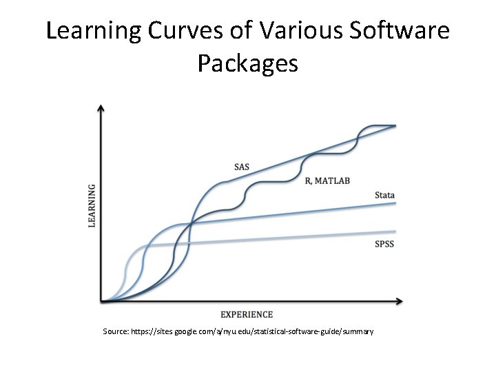
Learning Curves of Various Software Packages Source: https: //sites. google. com/a/nyu. edu/statistical-software-guide/summary

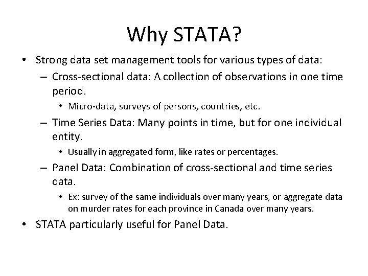
Why STATA? • Strong data set management tools for various types of data: – Cross-sectional data: A collection of observations in one time period. • Micro-data, surveys of persons, countries, etc. – Time Series Data: Many points in time, but for one individual entity. • Usually in aggregated form, like rates or percentages. – Panel Data: Combination of cross-sectional and time series data. • Ex: survey of the same individuals over many years, or aggregate data on murder rates for each province in Canada over many years. • STATA particularly useful for Panel Data.

Reading/Cleaning data

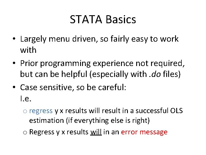
STATA Basics • Largely menu driven, so fairly easy to work with • Prior programming experience not required, but can be helpful (especially with. do files) • Case sensitive, so be careful: I. e. o regress y x results will result in a successful OLS estimation (if everything else is right) o Regress y x results will in an error message

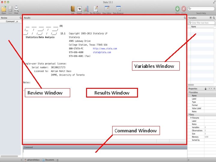
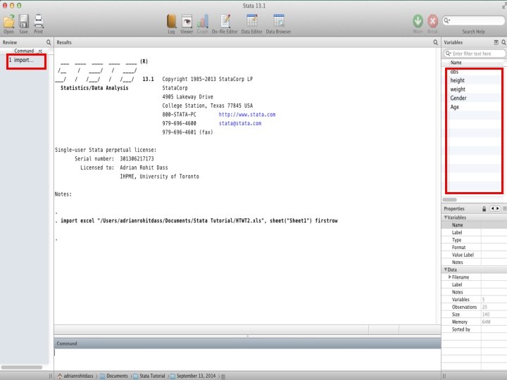
Variables Window Review Window Results Window Command Window

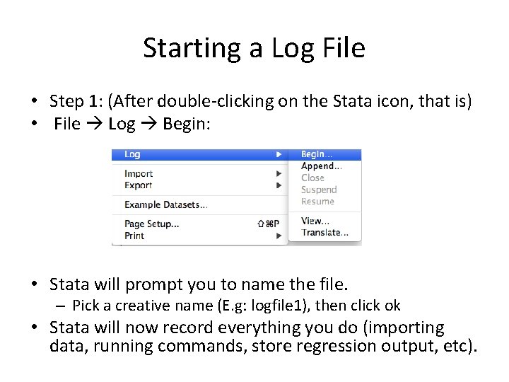
Starting a Log File • Step 1: (After double-clicking on the Stata icon, that is) • File Log Begin: • Stata will prompt you to name the file. – Pick a creative name (E. g: logfile 1), then click ok • Stata will now record everything you do (importing data, running commands, store regression output, etc).

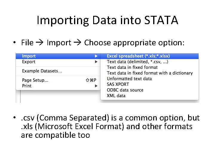
Importing Data into STATA • File Import Choose appropriate option: • . csv (Comma Separated) is a common option, but. xls (Microsoft Excel Format) and other formats are compatible too

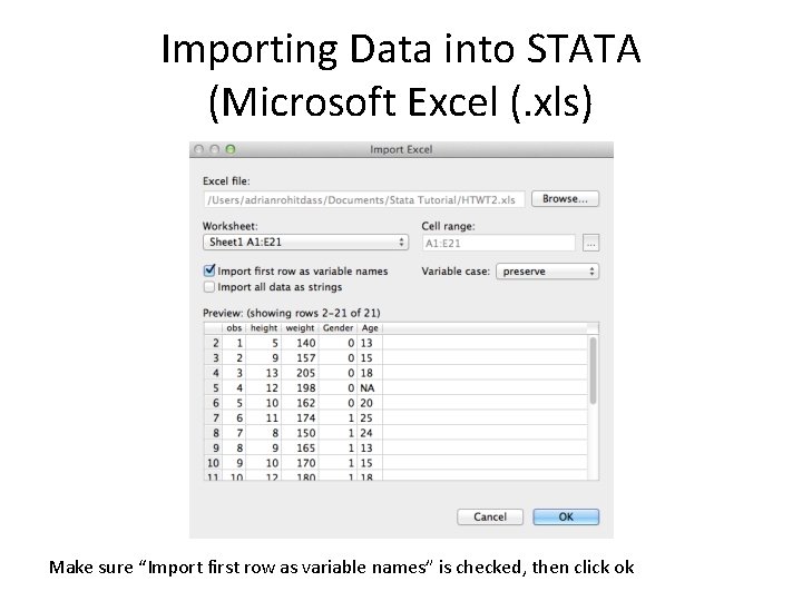
Importing Data into STATA (Microsoft Excel (. xls) Make sure “Import first row as variable names” is checked, then click ok

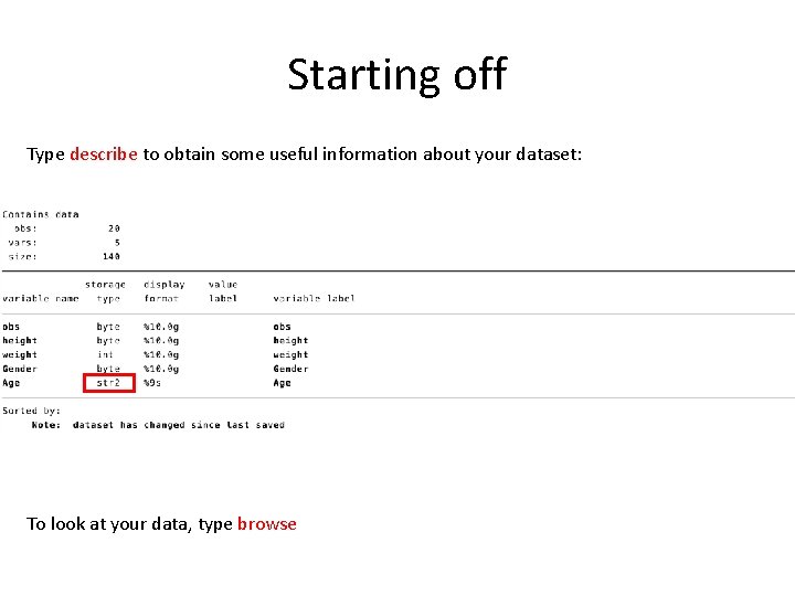
Starting off Type describe to obtain some useful information about your dataset: To look at your data, type browse

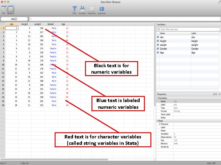
Black text is for numeric variables Blue text is labeled numeric variables Red text is for character variables (called string variables in Stata)

Convert Character variable to Numeric Make use of Stata’s destring command: destring [varlist] , {generate(newvarlist)|replace} [destring_options] Eg: destring Age, replace ignore(NA)

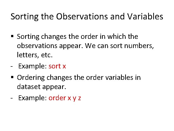
Sorting the Observations and Variables § Sorting changes the order in which the observations appear. We can sort numbers, letters, etc. - Example: sort x § Ordering changes the order variables in dataset appear. - Example: order x y z

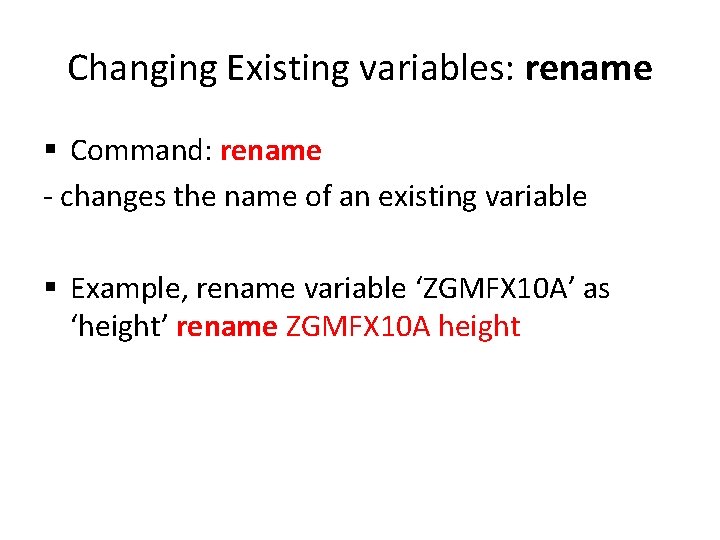
Changing Existing variables: rename § Command: rename - changes the name of an existing variable § Example, rename variable ‘ZGMFX 10 A’ as ‘height’ rename ZGMFX 10 A height

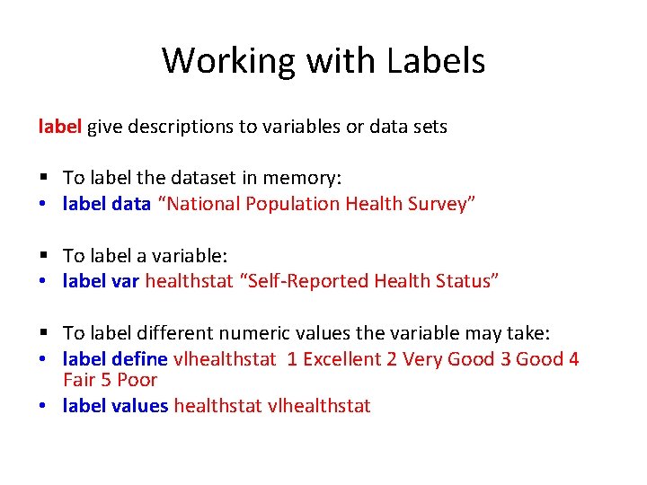
Working with Labels label give descriptions to variables or data sets § To label the dataset in memory: • label data “National Population Health Survey” § To label a variable: • label var healthstat “Self-Reported Health Status” § To label different numeric values the variable may take: • label define vlhealthstat 1 Excellent 2 Very Good 3 Good 4 Fair 5 Poor • label values healthstat vlhealthstat

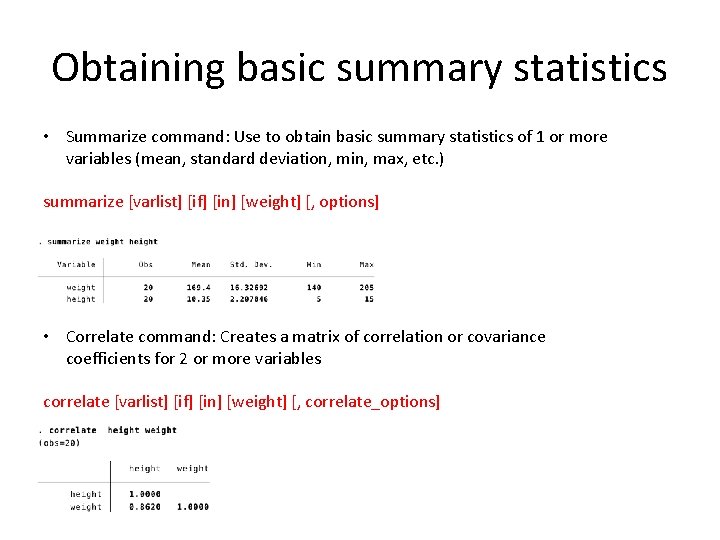
Obtaining basic summary statistics • Summarize command: Use to obtain basic summary statistics of 1 or more variables (mean, standard deviation, min, max, etc. ) summarize [varlist] [if] [in] [weight] [, options] • Correlate command: Creates a matrix of correlation or covariance coefficients for 2 or more variables correlate [varlist] [if] [in] [weight] [, correlate_options]

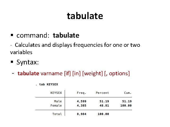
tabulate § command: tabulate - Calculates and displays frequencies for one or two variables § Syntax: - tabulate varname [if] [in] [weight] [, options]

More detailed descriptives • Use tabstat command tabstat varlist [if] [in] [weight] [, options] • This example calculates the sum of the variable • Default stat in tabstat is mean (no specification) • Other statistics: min, max, skewness, kurtosis. . .

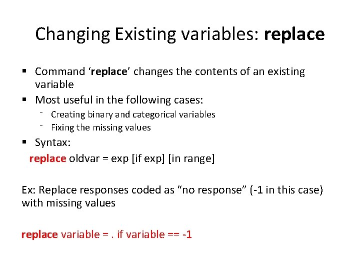
Changing Existing variables: replace § Command ‘replace’ changes the contents of an existing variable § Most useful in the following cases: ⁻ Creating binary and categorical variables ⁻ Fixing the missing values § Syntax: replace oldvar = exp [if exp] [in range] Ex: Replace responses coded as “no response” (-1 in this case) with missing values replace variable =. if variable == -1

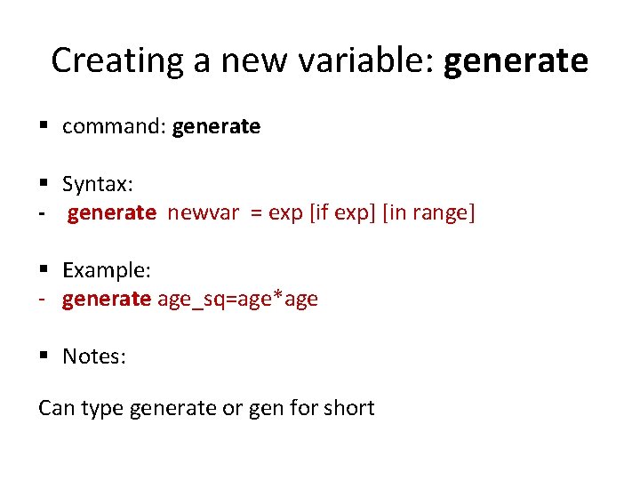
Creating a new variable: generate § command: generate § Syntax: - generate newvar = exp [if exp] [in range] § Example: - generate age_sq=age*age § Notes: Can type generate or gen for short

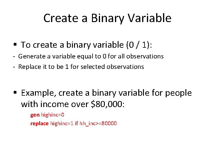
Create a Binary Variable § To create a binary variable (0 / 1): - Generate a variable equal to 0 for all observations - Replace it to be 1 for selected observations § Example, create a binary variable for people with income over $80, 000: gen highinc=0 replace highinc=1 if hh_inc>=80000

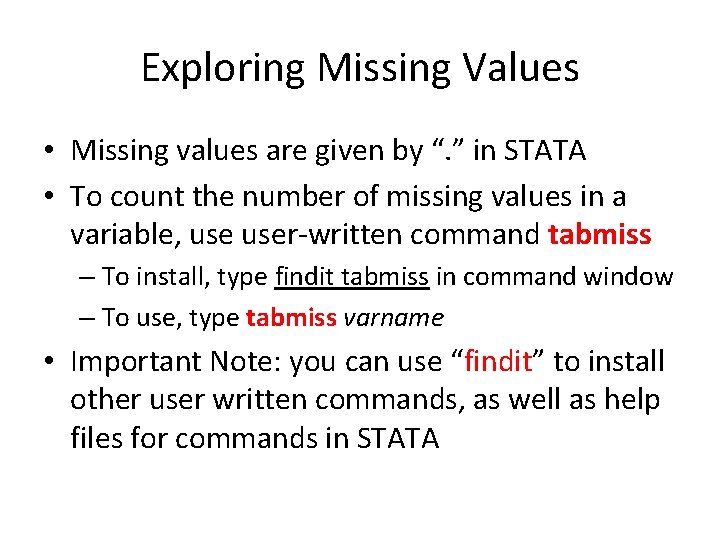
Exploring Missing Values • Missing values are given by “. ” in STATA • To count the number of missing values in a variable, user-written command tabmiss – To install, type findit tabmiss in command window – To use, type tabmiss varname • Important Note: you can use “findit” to install other user written commands, as well as help files for commands in STATA

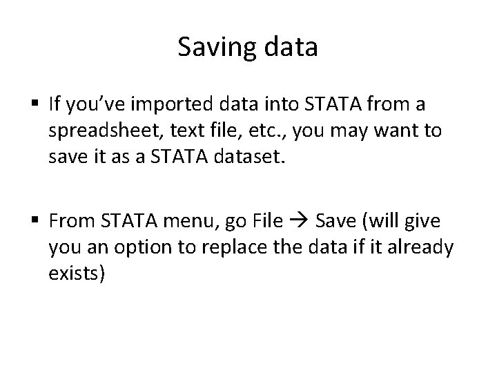
Saving data § If you’ve imported data into STATA from a spreadsheet, text file, etc. , you may want to save it as a STATA dataset. § From STATA menu, go File Save (will give you an option to replace the data if it already exists)

Graphing/Plotting Data • Plain Text Plot plot yvar 1 [yvar 2 [yvar 3]] xvar [if exp] [in range] [, columns(#) encode hlines(#) vlines(#) ] – ex: plot weight height • Graphics Plot (generates an image file) [graph] twoway plot [if] [in] [, twoway_options] – ex. graph twoway scatter weight height

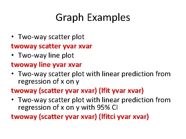
Graph Examples • Two-way scatter plot twoway scatter yvar xvar • Two-way line plot twoway line yvar xvar • Two-way scatter plot with linear prediction from regression of x on y twoway (scatter yvar xvar) (lfit yvar xvar) • Two-way scatter plot with linear prediction from regression of x on y with 95% CI twoway (scatter yvar xvar) (lfitci yvar xvar)

Regression Analysis

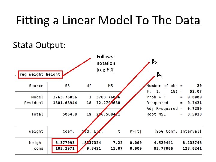
Fitting a Linear Model To The Data General notation: regress depvar [indepvars] [if] [in] [weight] [, options] Where: Y is our dependent variable X is our independent variable(s) Note: You may type “reg” instead of “regress” Determining which variables are what is usually determined by theory Research Question: Is there a relationship between weight and height?

Fitting a Linear Model To The Data Stata Output: Follows notation (reg Y X) β 2 β 1

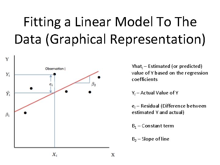
Fitting a Linear Model To The Data (Graphical Representation) Yhati – Estimated (or predicted) value of Y based on the regression coefficients Yi – Actual Value of Y ei – Residual (Difference between estimated Y and actual) B 1 – Constant term B 2 – Slope of line

Post Estimation

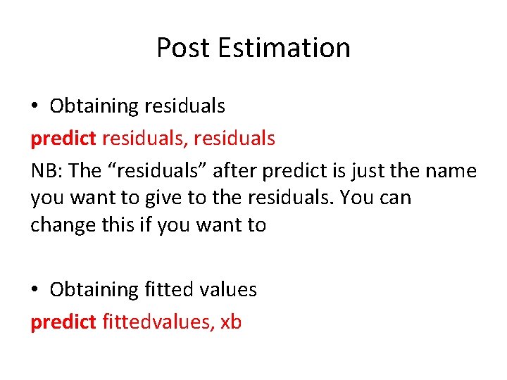
Post Estimation • Obtaining residuals predict residuals, residuals NB: The “residuals” after predict is just the name you want to give to the residuals. You can change this if you want to • Obtaining fitted values predict fittedvalues, xb

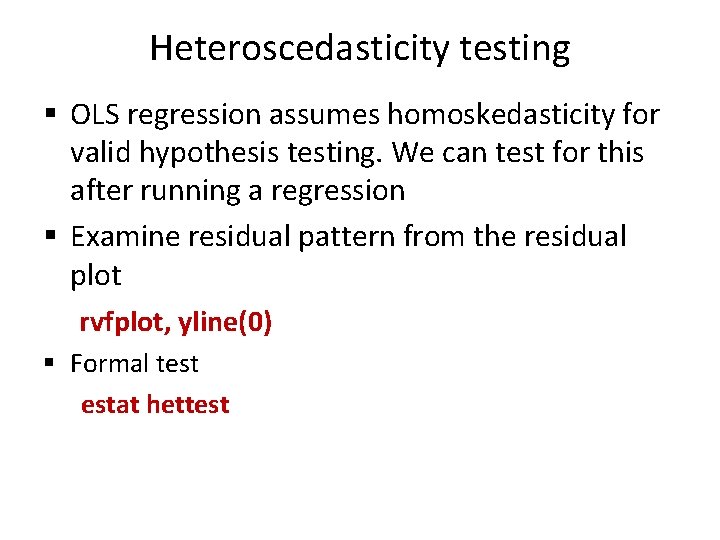
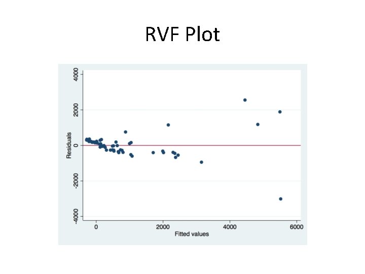
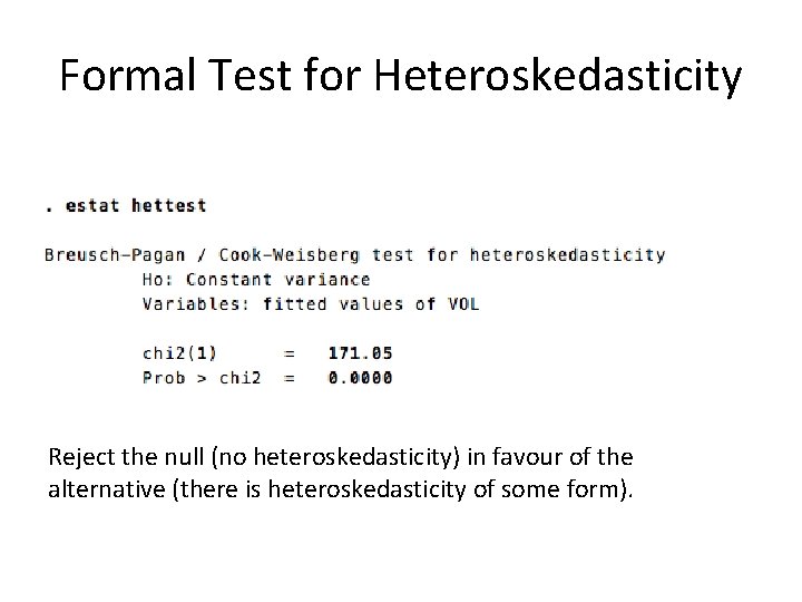
Heteroscedasticity testing § OLS regression assumes homoskedasticity for valid hypothesis testing. We can test for this after running a regression § Examine residual pattern from the residual plot rvfplot, yline(0) § Formal test estat hettest

RVF Plot

Formal Test for Heteroskedasticity Reject the null (no heteroskedasticity) in favour of the alternative (there is heteroskedasticity of some form).

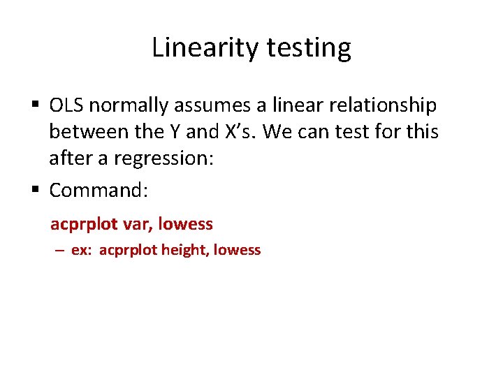
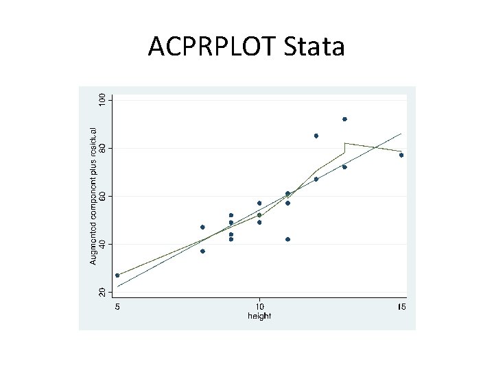
Linearity testing § OLS normally assumes a linear relationship between the Y and X’s. We can test for this after a regression: § Command: acprplot var, lowess – ex: acprplot height, lowess

ACPRPLOT Stata

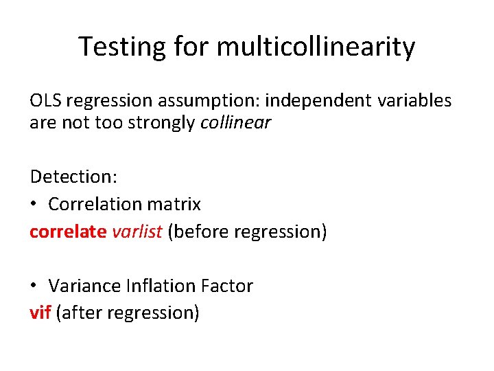
Testing for multicollinearity OLS regression assumption: independent variables are not too strongly collinear Detection: • Correlation matrix correlate varlist (before regression) • Variance Inflation Factor vif (after regression)

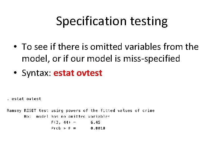
Specification testing • To see if there is omitted variables from the model, or if our model is miss-specified • Syntax: estat ovtest

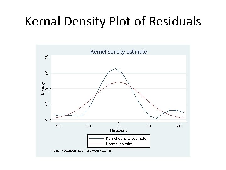
Testing Normality of Residuals § We assume that the errors are normally distributed for hypothesis testing. We can use the residuals to test this assumption. § Command predict r, residuals kdensity r, normal

Kernal Density Plot of Residuals

Parameter Hypothesis Testing • Test whether a parameter equal zero - testparm height - test (height) • Test both parameters equal zero - test (height weight) • Test if coefficients on two variables are equal - test (height= weight)

Storing Estimation Results • STATA can store the results of your regression via the estimates command: estimates store name • This can be very useful in analyzing regression results after running multiple models • To list multiple results side-by-side, type estimates table name 1 name 2…name 5, etc. • To export results from STATA to excel, word, or La. Te. X, user-written command esttab: http: //repec. org/bocode/e/estout/esttab. html

Advanced Topics in STATA

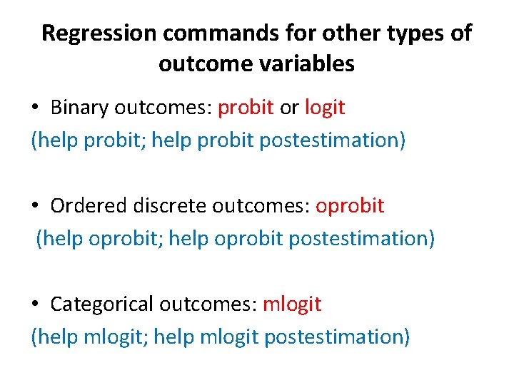
Regression commands for other types of outcome variables • Binary outcomes: probit or logit (help probit; help probit postestimation) • Ordered discrete outcomes: oprobit (help oprobit; help oprobit postestimation) • Categorical outcomes: mlogit (help mlogit; help mlogit postestimation)

Panel Data Econometrics • Pooled Linear Regress regress depvar [indepvars] [if] [in] [weight] [, options] • Random Effects xtreg depvar [indepvars] [if] [in] [, re RE_options] • Fixed Effects xtreg depvar [indepvars] [if] [in] [weight] , fe [FE_options]

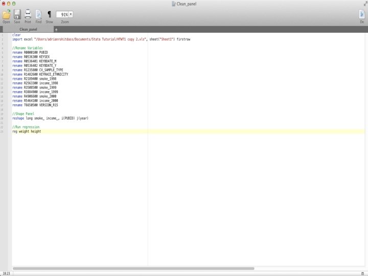
Working With Do-Files Motivation Why bother? 1) We can ovoid tediously running the same set of commands over and over again… 2) Creates a document listing all the commands we’ve run in plain text form 3) Increases our productivity with STATA!

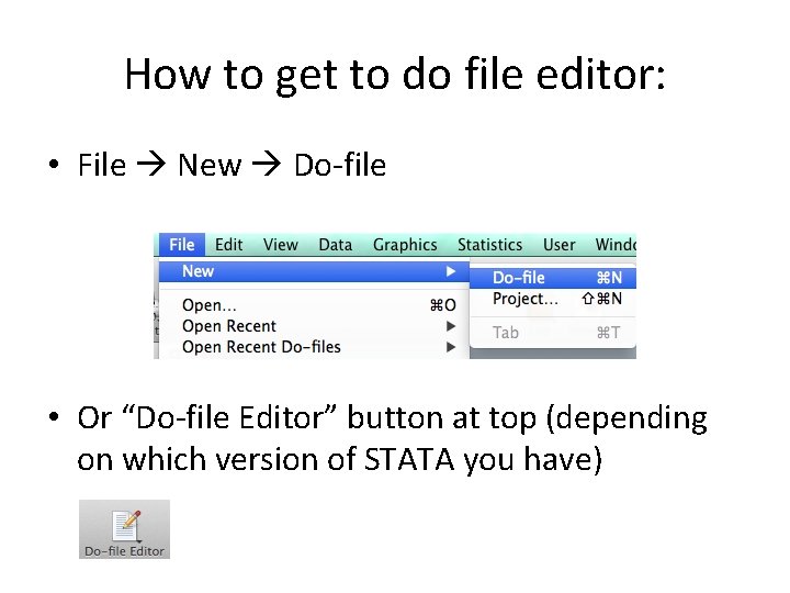
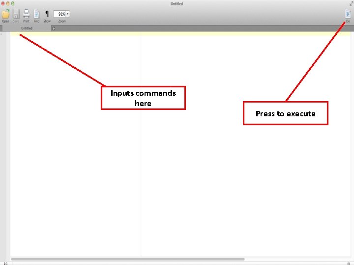
How to get to do file editor: • File New Do-file • Or “Do-file Editor” button at top (depending on which version of STATA you have)

Inputs commands here Press to execute

STATA Resources

STATA Online Resources • STATA manuals are freely downloadable from the above site http: //www. statapress. com/manuals/documentation-set/ • Typing help [topic] in the command window is also useful, but the online manuals generally contain more detail/examples

STATA Online Resources UCLA Institute for Digital Research and Education • List of topics and STATA resources can be found here: http: //www. ats. ucla. edu/stata/webbooks/r eg/default. htm

Other STATA Resources • Jones, A. M. , Rice, N. , d’Uva, T. B. , Balia, S. 2013. Applied Health Economics - Second Edition, Routledge Advanced Texts in Economics and Finance. Taylor & Francis • Cameron, A. C. , Trivedi, P. K. 2010. Microeconometrics Using Stata – Revised Edition, Stata Press books. • Allison, P. D. 2009. Fixed Effects Regression Models, Quantitative Applications in the Social Sciences. SAGE Publications.

Useful sites to find and download Canadian data • Ontario Data Documentation, Extraction Service and Infrastructure (ODESI) website: http: //search 2. odesi. ca/ • Computing in the Humanities and Social Sciences (CHASS) at U of T http: //www. chass. utoronto. ca

Thanks for Listening Good luck with STATA!