Teoria podejmowania decyzji Wykad 7 Reduction of compound

Teoria podejmowania decyzji Wykład 7

Reduction of compound lotteries 1 A 1/2 1/3 1/3 1/4 3/8 A B 1/2 1/2 A B C 1/4 3/8 A 1/2 B C 1/2 1/4 A B C A C

Von Neumann Morgenstern proof graphically 1

Von Neumann Morgenstern proof graphically 2

Common misunderstandings

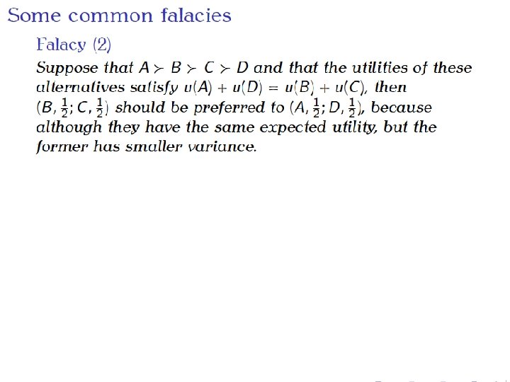
Fallacy (2) • Fire insurance: – Fire: pay the premium, house rebuilt (C) – No Fire: pay the premium, house untouched (B) Loss = $70 K Loss = $60 K – Fire: house burnt, no compansation (D) – No Fire: house the same (A) Loss = $100 K Loss = $0 • No insurance: • A≻B≻C≻D • Suppose the probability of fire is 0. 5 • And an individual is indifferent between buying and not buying the insurance • Although Fire insurance has smaller variance and ½u(A) + ½u(D) = ½u(B) + ½u(C), it does not mean that Fire insurance should be chosen over No insurance Risk averse, and EL(insurance) = $65 K EL(no insurance) = $50 K

Fallacy (3) • Fire insurance: – Fire: pay the premium, house rebuilt (C) – No Fire: pay the premium, house untouched (B) • No insurance: – Fire: house burnt, no compansation (D) – No Fire: house the same (A) • A≻B≻C≻D • Suppose that the probability of fire is ½ and an individual prefers not buying fire insurance and hence ½u(A) + ½u(D) > ½u(B) + ½u(C) ⇒ u(A) - u(B) > u(C) - u(D) • However it does not mean that the change from B to A is more preferred than the change from D to C. • Preferences are defined over pairs of alternatives not pairs of alternatives

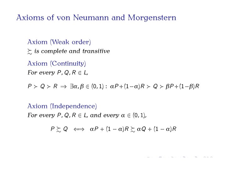
Crucial axiom - independence • Our version • The general version • Why the general version implies our version?

Independence – examples • If I prefer to go to the movies than to go for a swim, I must prefer: – to toss a coin and: • heads: go to the movies • tails: vacuum clean – than to toss a coin and: • heads: go for a swim • tails: vacuum clean • If I prefer to bet on red than on even in roulette, then I must prefer: – to toss a coin and • heads: bet on 18 • tails: bet on red – than to toss a coin and: • heads: bet on 18 • tails: bet on even 14

Machina triangle p 2 1 a 1 - a x 2 x 3 R P a. P +(1 -a)R x 1 1 p 1 15

Independence assumption in the Machina triangle Suppose that A 1 is better than A 2 is better than A 3 p 2 1 αP+(1 -α)R R αQ+(1 -α)R P Q 1 p 1 16

17. 1 and 17. 2 17. 1) Choose one lottery: P=(1 mln, 1) Q=(5 mln, 0. 1; 1 mln, 0. 89; 0 mln, 0. 01) 17. 2) Choose one lottery: P’=(1 mln, 0. 11; 0 mln, 0. 89) Q’=(5 mln, 0. 1; 0 mln, 0. 9) Kahneman, Tversky (1979) [common consequence effect violation of independence] Many people choose P over Q and Q’ over P’

Common consequence graphically P = (1 mln, 1) P’= (1 mln, 0. 11; 0, 0. 89) Q = (5 mln, 0. 1; 1 mln, 0. 89; 0, 0. 01) Q’= (5 mln, 0. 1; 0, 0. 9) • If we plug c = 1 mln, we get P and Q respectively • If we plug c = 0, we get P’ and Q’ respectively

18. 1 i 18. 2 18. 1) Choose one lottery: P=(3000 PLN, 1) Q=(4000 PLN, 0. 8; 0 PLN, 0. 2) 18. 2) Choose one lottery: P’=(3000 PLN, 0. 25; 0 PLN, 0. 75) Q’=(4000 PLN, 0. 2; 0 PLN, 0. 8) Kahneman, Tversky (1979) [common ratio effect, violation of independence] Many people choose P over Q and Q’ over P’

Common ratio graphically P=(3000 PLN, 1) P’=(3000 PLN, 0. 25; 0 PLN, 0. 75) Q=(4000 PLN, 0. 8; 0 PLN, 0. 2) Q’=(4000 PLN, 0. 2; 0 PLN, 0. 8)

Monotonicity of utility function 21 Behaviour x+d x Prefers more to less

Monotonicity of utility function 22 Behaviour Utility function Prefers more to less x, u’(x)>0; u(x) – increasing

Monotonicity of utility function 23 Behaviour Utility function Prefers more to less x, u’(x)>0; u(x) – increasing Attitude towards risk (quantitatively) u(x)/u’(x) – fear of ruin • prefers more to less • current wealth x • probability p of bankruptcy (u(0)=0) • how much to pay to avoid it?

Monotonicity of utility function 24 Behaviour Utility function Prefers more to less x, u’(x)>0; u(x) – increasing Attitude towards risk (quantitatively) u(x)/u’(x) – fear of ruin When is the choice obvious First order stochastic dominance (comparing cdf) – FOSD F(x) 1 x

Examples – comparing pairs of lotteries Payoff Pr. 1 50% 4 10% 1 50% 2 30% 5 50% 2 30% 3 20% 6 40% 3 20% 4 20% Payoff Pr. 1 50% 1 40% 2 30% 2 35% 3 20% 3 30% 3 25%

First Order Stochastic Dominance (FOSD) cdf Payoff Pr. 1 50% 4 10% 2 30% 5 50% 3 20% 6 40% 1 1 t cdf Payoff Pr. 1 50% 1 40% 2 35% 3 20% 3 25% 1

FOSD • Assume X and Y are two different lotteries (FX(. ), FY(. ) are not the same) • Lottery X FOSD Y if: For all a, hence: Those who prefer more to less will never choose lottery that is dominated in the above sense. • Theorem: X FOSD Y if and only if Eu(X) ≥ Eu(Y), for all inreasing u

Compare Payoff Pr. 1 50% 1 40% 2 30% 2 50% 3 20% 3 30% 3 20% 3 10% Payoff Pr. 1 10% 0 30% 1 50% 2 90% 2 70% 2 55% 2 30% 3 5% 3 20% 4 15% 3 20% 4 5%

Marginal utility 29 Behaviour Risk averse, ie. Var(L)>0 u(E(L))>E(u(L)) x+d Today chance nodes split 50: 50 x-d x

Marginal utility 30 Behaviour utility Utility function payoff Risk averse, ie. Var(L)>0 u(E(L))>E(u(L)) x, u’(x)>0, u’’(x)<0; u(x) – concave, increasing

Certainty equivalent and risk premium 1 4, 5 2 utility 0, 5 1 10 6

Marginal utility 32 Behaviour Utility function Risk averse, ie. Var(L)>0 u(E(L))>E(u(L)) x, u’(x)>0, u’’(x)<0; u(x) – concave, increasing Attitude towards risk (quantitatively) -u’’(x)/u’(x) – Arrow-Pratt risk aversion coeff. • • • x – initial wealth (number) l – lottery with zero exp. value (random variable) k – multiplier (we tak k close to zero) d – risk premium (number) x-d – certainty equivalent for x+l

Marginal utility 33 Behaviour Utility function Risk averse, ie. Var(L)>0 u(E(L))>E(u(L)) x, u’(x)>0, u’’(x)<0; u(x) – concave, increasing Attitude towards risk (quantitatively) -u’’(x)/u’(x) – Arrow-Pratt risk aversion coeff. When is the choice obvious Second order stochastic dominance (integrals of cdf) – SOSD

Second Order Stochastic Dominance cdf Payoff Pr. 1 30% 1 50% 2 60% 2 20% 3 10% 3 30% 1 1 t F(x) Sum 1 0, 3 0 1 0, 5 0 2 0, 9 0, 3 2 0, 7 0, 5 3 1 1, 2 4 1 2, 2 t 1 1 t

SOSD • Assume X and Y are two different lotteries (FX(. ), FY(. ) are not the same) • Lottery X SOSD Y if: For all a hence: • Those who are risk averse will never choose a lottery that is dominated in the above sense. • Theorem: X SOSD Y if and only if Eu(X) ≥ Eu(Y), for all inreasing and concave u

Compare and find FOSD and SOSD Payoff Pr. 1 50% 1 60% 1 15% 1 20% 2 30% 2 10% 2 45% 2 40% 3 20% 3 30% 3 40% Payoff Pr. 1 10% 1 30% 1 40% 2 50% 2 15% 2 40% 2 15% 3 40% 3 55% 3 30% 3 45%

Mean-variance criterium • Risk aversion doesn’t mean that always: A better than B, if only E(A)=E(B) and Var(A)<Var(B) – some lotteries do not result from another with mean preserving spread – is true when Var(A)=0 • Mean-variance criterium works e. g. for normally distributed random variables (lotteries) Lottery X Lottery Y Prob. x u(x)=ln(x) (x-EX)2 y u(y)=ln(y) (y-EY)2 20% 20, 1 3 65, 61 4 1, 386 64 80% 9, 975 2, 3 4, 1 14 2, 639 4 mean 12 2, 44 16, 4 12 2, 388 16 37

Measures of risk aversion • Risk premium measures risk aversion with respect to a given lottery • As a function of payoff values risk aversion is measured by Arrow, Pratt measures of (local) risk aversion

25 20 15 10 5 0 0 5 10 15 20

Exercise 1 • From now on let’s assume X is a set of monetary payoffs (decision maker prefers more money than less) • Decision maker with v. NM utility function prefers lottery (100, ¼; 1000, ¾) to (500, ½; 1000, ½) • What is a realtion between (100, ½; 500, ¼; 1000, ¼) and (100, ¼; 500, ¾)? • Suggestion – we can arbitrarily set utility function for two outcomes 41

Exercise 2 • Decision maker is indifferent between pairs of lotteries: (500, 1) and (0, 0, 4; 1000, 0, 6) and (300, 1) and (0, ½; 500, ½) • Can we guess the preference relation between (0, 0, 2; 300, 0, 3; 1000, ½) and (500, 1)? 42

Exercise 3 • Decision maker with v. NM utility is risk averse and indifferent between the following pairs (400, 1) and (0, 0, 3; 1000, 0, 7) and (0, ½; 200, ½) and (0, 5/7; 400, 2/7) • Can we guess the preference relation between (200, ½; 600, ½) and (0, 4/9; 100, 5/9)? • (suggestion – remamber than v. NM utility is concave) 43