Support Vector Machine SVM v MUMT 611 v

Support Vector Machine (SVM) v MUMT 611 v Beinan Li v Music Tech @ Mc. Gill v 2005 -3 -17 1

Content v Related problems in pattern classification v VC theory and VC dimension v Overview of SVM v Application example 2

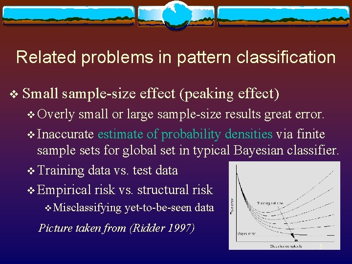
Related problems in pattern classification v Small sample-size effect (peaking effect) v Overly small or large sample-size results great error. v Inaccurate estimate of probability densities via finite sample sets for global set in typical Bayesian classifier. v Training data vs. test data v Empirical risk vs. structural risk v Misclassifying yet-to-be-seen data Picture taken from (Ridder 1997) 3

Related problems in pattern classification v Avoid solving a more general problem as an intermediate step. (Vapnik 1995) v Do it without estimation of probability of densities. v ANN v Depends on knowledge v Empirical-risk method (ERM): v Problem v To of generalization (hard to control over-fitting) find theoretical analysis for validity of ERM. 4

VC theory and VC dimension v VC dimension: (classifier complexity) v The maximum size of a sample set that a decision function can separate. v Finite VC dimension coherence of ERM v Theoretical v Linear v VC decision function: dim = number of parameters v Non-linear v VC basis of ANN and SVM decision function: dim <= number of parameters 5

Overview of SVM v Structural-risk method (SRM) v Minimize ER v Control VC dimension v Result: tradeoff between ER and over-fitting v Focus v To on the explicit problem of classification: find the optimal hyperplane for dividing two classes v Supervised learning 6

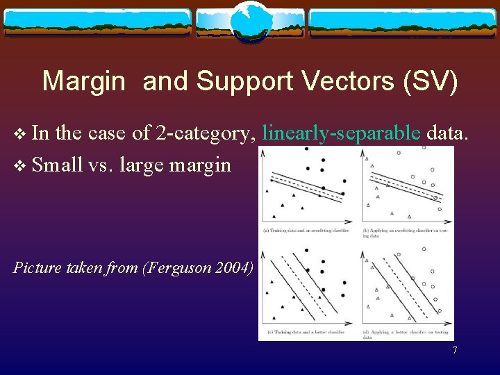
Margin and Support Vectors (SV) v In the case of 2 -category, linearly-separable data. v Small vs. large margin Picture taken from (Ferguson 2004) 7

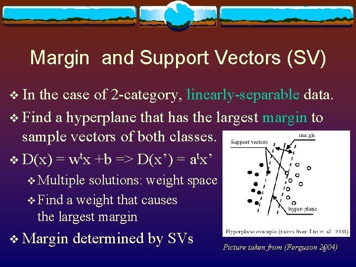
Margin and Support Vectors (SV) v In the case of 2 -category, linearly-separable data. v Find a hyperplane that has the largest margin to sample vectors of both classes. v D(x) = wtx +b => D(x’) = atx’ v Multiple solutions: weight space v Find a weight that causes the largest margin v Margin determined by SVs Picture taken from (Ferguson 2004) 8

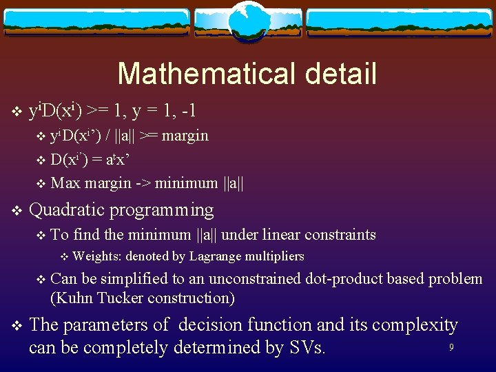
Mathematical detail v yi. D(xi) >= 1, y = 1, -1 v yi. D(xi’) / ||a|| >= margin v D(xi’) = atx’ v Max margin -> minimum ||a|| v Quadratic programming v To find the minimum ||a|| under linear constraints v Weights: v v denoted by Lagrange multipliers Can be simplified to an unconstrained dot-product based problem (Kuhn Tucker construction) The parameters of decision function and its complexity 9 can be completely determined by SVs.

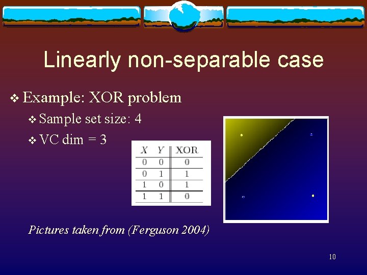
Linearly non-separable case v Example: XOR problem v Sample set size: 4 v VC dim = 3 Pictures taken from (Ferguson 2004) 10

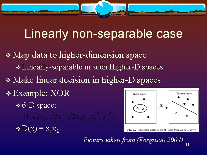
Linearly non-separable case v Map data to higher-dimension space v Linearly-separable in such Higher-D spaces v Make linear decision in higher-D spaces v Example: XOR v 6 -D space: v D(x) = x 1 x 2 Picture taken from (Ferguson 2004) 11

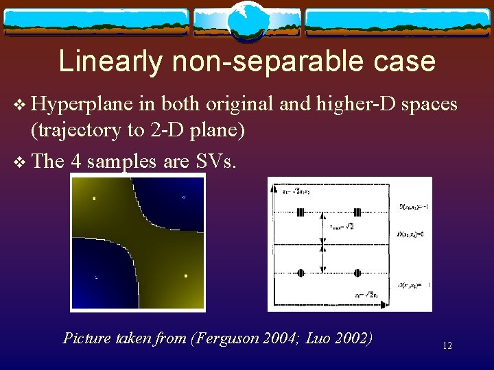
Linearly non-separable case v Hyperplane in both original and higher-D spaces (trajectory to 2 -D plane) v The 4 samples are SVs. Picture taken from (Ferguson 2004; Luo 2002) 12

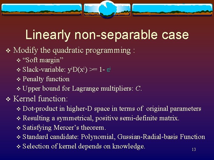
Linearly non-separable case v Modify the quadratic programming : “Soft margin” v Slack-variable: yi. D(xi) >= 1 - εi v Penalty function v Upper bound for Lagrange multipliers: C. v v Kernel function: Dot-product in higher-D space in terms of original parameters v Resulting a symmetrical, positive semi-definite matrix. v Satisfying Mercer’s theorem. v Standard candidate: Polynomial, Gussian-Radial-basis Function v Selection of kernel depends on knowledge. 13 v

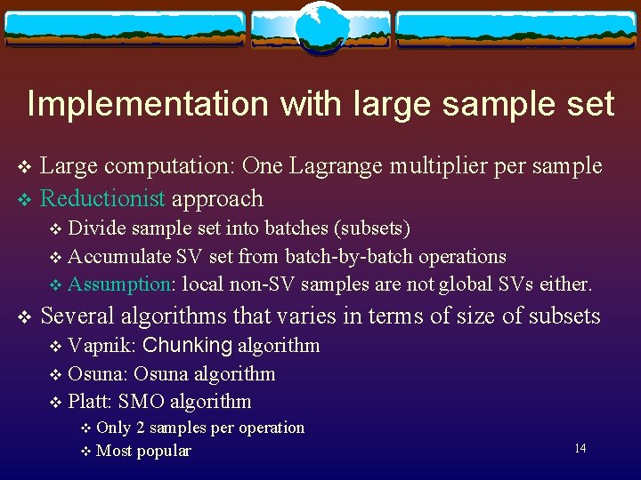
Implementation with large sample set Large computation: One Lagrange multiplier per sample v Reductionist approach v Divide sample set into batches (subsets) v Accumulate SV set from batch-by-batch operations v Assumption: local non-SV samples are not global SVs either. v v Several algorithms that varies in terms of size of subsets Vapnik: Chunking algorithm v Osuna: Osuna algorithm v Platt: SMO algorithm v v Only 2 samples per operation v Most popular 14

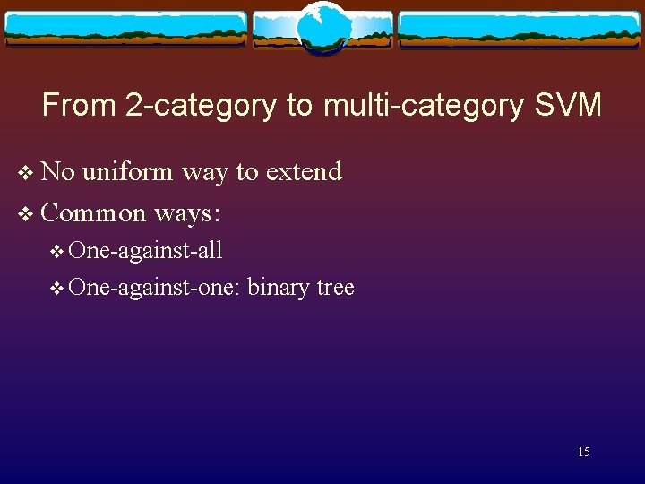
From 2 -category to multi-category SVM v No uniform way to extend v Common ways: v One-against-all v One-against-one: binary tree 15

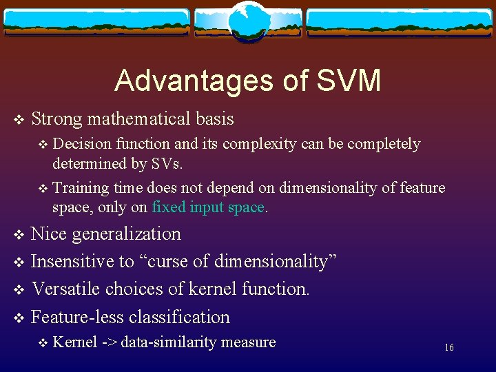
Advantages of SVM v Strong mathematical basis Decision function and its complexity can be completely determined by SVs. v Training time does not depend on dimensionality of feature space, only on fixed input space. v Nice generalization v Insensitive to “curse of dimensionality” v Versatile choices of kernel function. v Feature-less classification v v Kernel -> data-similarity measure 16

Drawback of SVM v Still rely on knowledge Choices of C, kernel and penalty function v C: how far the decision function is adapted to avoid any error v Kernel: how much freedom SVM should adapt itself (dimension) v v Overlapping classes Reductionism may discard promising SVs at any batch step. v The classification can be limited by the size of the problem. v No uniform way to extend 2 -category to multi-category 17 v “Still not an ideal optimally-generalizing classifier. ” v

Applications v Vapnik et al. at AT&T: v Handwritten number recognition v Error rate is lower than that of ANN v Speech recognition v Face recognition v MIR v SVM-light: open source C library 18

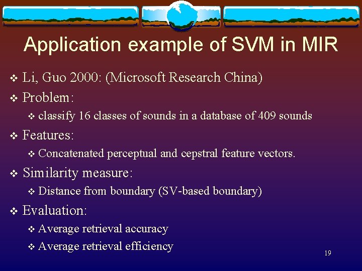
Application example of SVM in MIR Li, Guo 2000: (Microsoft Research China) v Problem: v v v Features: v v Concatenated perceptual and cepstral feature vectors. Similarity measure: v v classify 16 classes of sounds in a database of 409 sounds Distance from boundary (SV-based boundary) Evaluation: Average retrieval accuracy v Average retrieval efficiency v 19

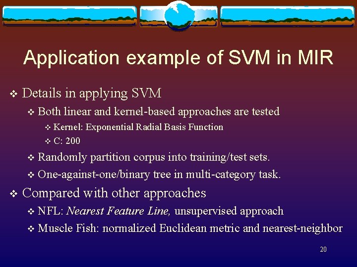
Application example of SVM in MIR v Details in applying SVM v Both linear and kernel-based approaches are tested v Kernel: v C: Exponential Radial Basis Function 200 Randomly partition corpus into training/test sets. v One-against-one/binary tree in multi-category task. v v Compared with other approaches NFL: Nearest Feature Line, unsupervised approach v Muscle Fish: normalized Euclidean metric and nearest-neighbor v 20

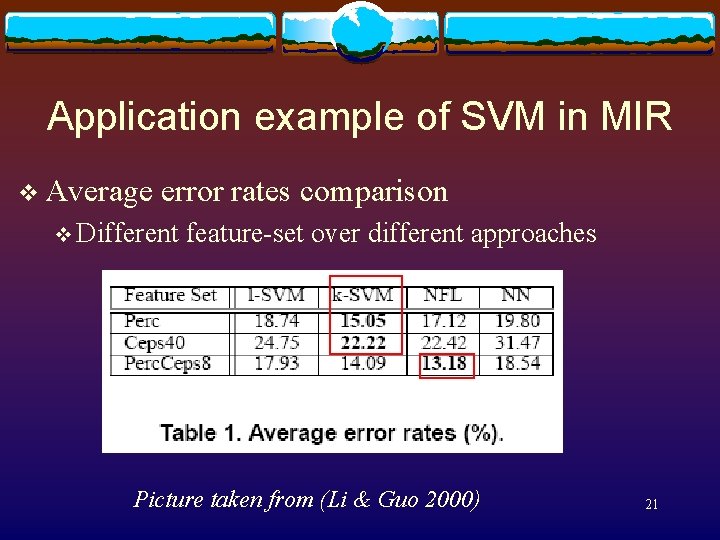
Application example of SVM in MIR v Average error rates comparison v Different feature-set over different approaches Picture taken from (Li & Guo 2000) 21

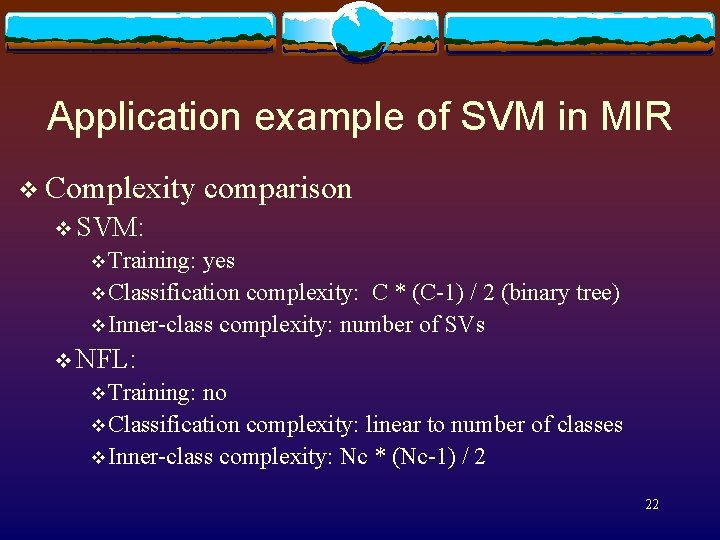
Application example of SVM in MIR v Complexity comparison v SVM: v Training: yes v Classification complexity: C * (C-1) / 2 (binary tree) v Inner-class complexity: number of SVs v NFL: v Training: no v Classification complexity: linear to number of classes v Inner-class complexity: Nc * (Nc-1) / 2 22

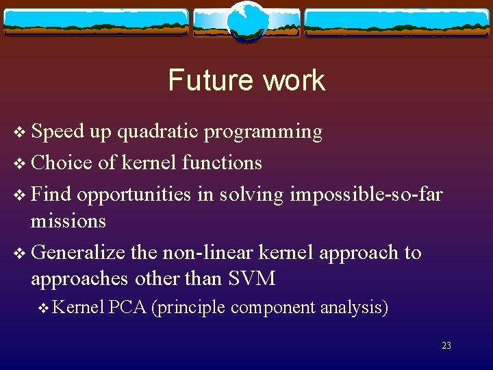
Future work v Speed up quadratic programming v Choice of kernel functions v Find opportunities in solving impossible-so-far missions v Generalize the non-linear kernel approach to approaches other than SVM v Kernel PCA (principle component analysis) 23

Bibliography v Summary: v http: //www. music. mcgill. ca/~damonli/MUMT 611/wee k 9_summary. pdf v HTML bibliography: v http: //www. music. mcgill. ca/~damonli/MUMT 611/wee k 9_bib. htm 24