A Simple Introduction to Support Vector Machines Martin

A Simple Introduction to Support Vector Machines Martin Law Lecture for CSE 802 Department of Computer Science and Engineering Michigan State University CSE 802. Prepared by Martin Law

Outline A brief history of SVM n Large-margin linear classifier n Linear separable n Nonlinear separable n Creating nonlinear classifiers: kernel trick n A simple example n Discussion on SVM n Conclusion n 10/26/2020 CSE 802. Prepared by Martin Law 2

History of SVM is related to statistical learning theory [3] n SVM was first introduced in 1992 [1] n SVM becomes popular because of its success in handwritten digit recognition n n 1. 1% test error rate for SVM. This is the same as the error rates of a carefully constructed neural network, Le. Net 4. n n See Section 5. 11 in [2] or the discussion in [3] for details SVM is now regarded as an important example of “kernel methods”, one of the key area in machine learning Note: the meaning of “kernel” is different from the “kernel” for Parzen [1] B. E. Boser etfunction al. A Training Algorithm for Optimalwindows Margin Classifiers. Proceedings of the Fifth Annual Workshop on n Computational Learning Theory 5 144 -152, Pittsburgh, 1992. [2] L. Bottou et al. Comparison of classifier methods: a case study in handwritten digit recognition. Proceedings of the 12 th IAPR International Conference on Pattern Recognition, vol. 2, pp. 77 -82. [3] V. Vapnik. The Nature of Statistical Learning Theory. 2 nd edition, Springer, 1999. 10/26/2020 CSE 802. Prepared by Martin Law 3

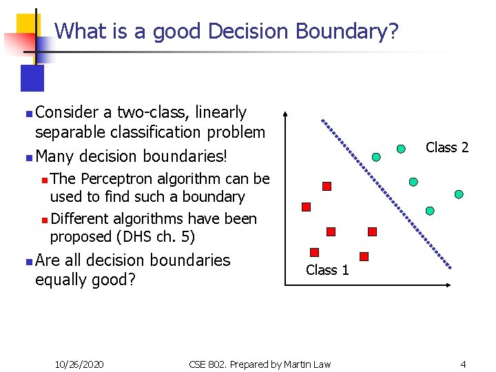
What is a good Decision Boundary? Consider a two-class, linearly separable classification problem n Many decision boundaries! n Class 2 The Perceptron algorithm can be used to find such a boundary n Different algorithms have been proposed (DHS ch. 5) n n Are all decision boundaries equally good? 10/26/2020 Class 1 CSE 802. Prepared by Martin Law 4

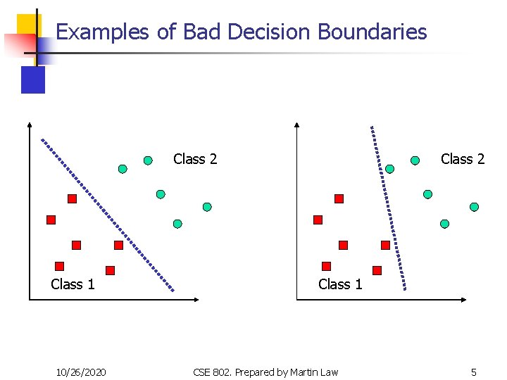
Examples of Bad Decision Boundaries Class 2 Class 1 10/26/2020 Class 2 Class 1 CSE 802. Prepared by Martin Law 5

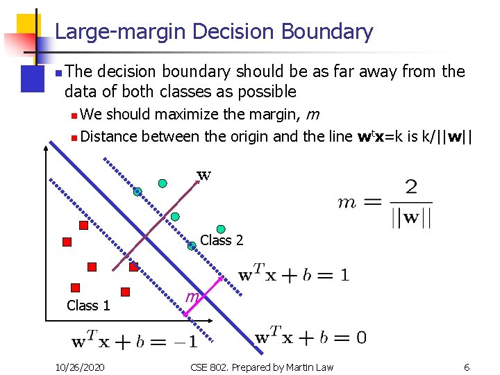
Large-margin Decision Boundary n The decision boundary should be as far away from the data of both classes as possible n We should maximize the margin, m n Distance between the origin and the line wtx=k is k/||w|| Class 2 Class 1 10/26/2020 m CSE 802. Prepared by Martin Law 6

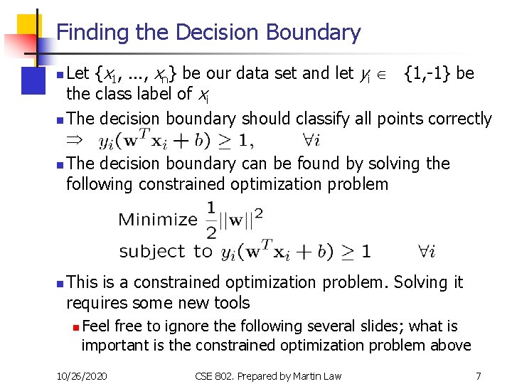
Finding the Decision Boundary Let {x 1, . . . , xn} be our data set and let yi Î {1, -1} be the class label of xi n The decision boundary should classify all points correctly n The decision boundary can be found by solving the following constrained optimization problem n n This is a constrained optimization problem. Solving it requires some new tools n Feel free to ignore the following several slides; what is important is the constrained optimization problem above 10/26/2020 CSE 802. Prepared by Martin Law 7

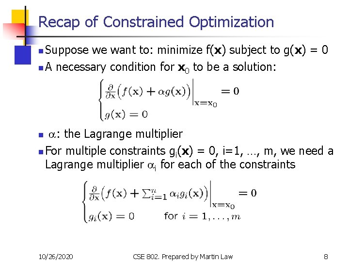
Recap of Constrained Optimization Suppose we want to: minimize f(x) subject to g(x) = 0 n A necessary condition for x 0 to be a solution: n a: the Lagrange multiplier n For multiple constraints gi(x) = 0, i=1, …, m, we need a Lagrange multiplier ai for each of the constraints n 10/26/2020 CSE 802. Prepared by Martin Law 8

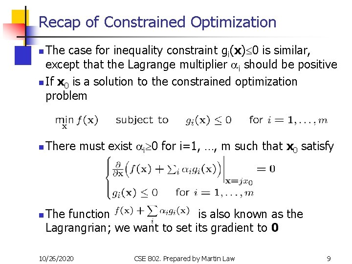
Recap of Constrained Optimization The case for inequality constraint gi(x)£ 0 is similar, except that the Lagrange multiplier ai should be positive n If x 0 is a solution to the constrained optimization problem n n n There must exist ai³ 0 for i=1, …, m such that x 0 satisfy The function is also known as the Lagrangrian; we want to set its gradient to 0 10/26/2020 CSE 802. Prepared by Martin Law 9

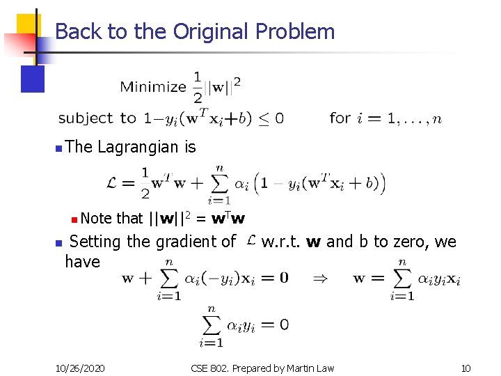
Back to the Original Problem n The Lagrangian is n n Note that ||w||2 = w. Tw Setting the gradient of have 10/26/2020 w. r. t. w and b to zero, we CSE 802. Prepared by Martin Law 10

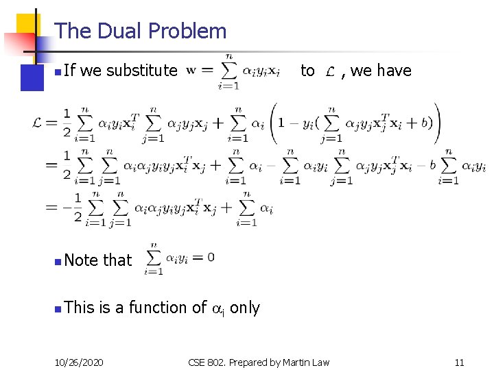
The Dual Problem n If we substitute n Note that n This is a function of ai only 10/26/2020 to CSE 802. Prepared by Martin Law , we have 11

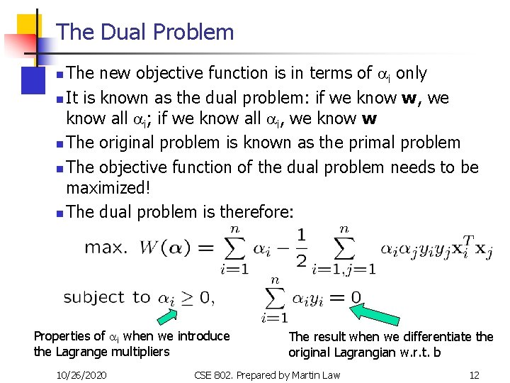
The Dual Problem The new objective function is in terms of ai only n It is known as the dual problem: if we know w, we know all ai; if we know all ai, we know w n The original problem is known as the primal problem n The objective function of the dual problem needs to be maximized! n The dual problem is therefore: n Properties of ai when we introduce the Lagrange multipliers 10/26/2020 The result when we differentiate the original Lagrangian w. r. t. b CSE 802. Prepared by Martin Law 12

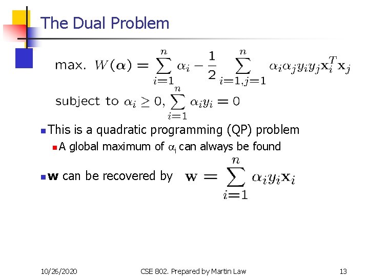
The Dual Problem n This is a quadratic programming (QP) problem n n A global maximum of ai can always be found w can be recovered by 10/26/2020 CSE 802. Prepared by Martin Law 13

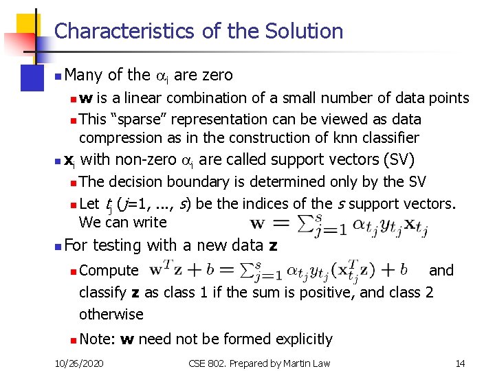
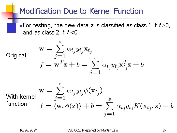
Characteristics of the Solution n Many of the ai are zero w is a linear combination of a small number of data points n This “sparse” representation can be viewed as data compression as in the construction of knn classifier n xi with non-zero ai are called support vectors (SV) n The decision boundary is determined only by the SV n Let tj (j=1, . . . , s) be the indices of the s support vectors. We can write n n For testing with a new data z n n Compute and classify z as class 1 if the sum is positive, and class 2 otherwise Note: w need not be formed explicitly 10/26/2020 CSE 802. Prepared by Martin Law 14

The Quadratic Programming Problem n Many approaches have been proposed n n Loqo, cplex, etc. (see http: //www. numerical. rl. ac. uk/qp/qp. html) Most are “interior-point” methods Start with an initial solution that can violate the constraints n Improve this solution by optimizing the objective function and/or reducing the amount of constraint violation n n For SVM, sequential minimal optimization (SMO) seems to be the most popular A QP with two variables is trivial to solve n Each iteration of SMO picks a pair of (ai, aj) and solve the QP with these two variables; repeat until convergence n n In practice, we can just regard the QP solver as a “black -box” without bothering how it works 10/26/2020 CSE 802. Prepared by Martin Law 15

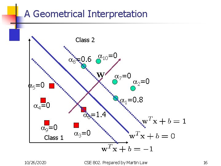
A Geometrical Interpretation Class 2 a 8=0. 6 a 10=0 a 7=0 a 5=0 a 4=0 a 9=0 Class 1 10/26/2020 a 2=0 a 1=0. 8 a 6=1. 4 a 3=0 CSE 802. Prepared by Martin Law 16

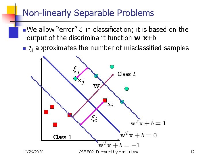
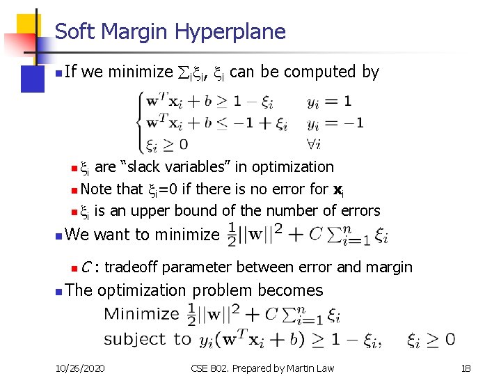
Non-linearly Separable Problems We allow “error” xi in classification; it is based on the output of the discriminant function w. Tx+b n xi approximates the number of misclassified samples n Class 2 Class 1 10/26/2020 CSE 802. Prepared by Martin Law 17

Soft Margin Hyperplane n If we minimize åixi, xi can be computed by xi are “slack variables” in optimization n Note that xi=0 if there is no error for xi n xi is an upper bound of the number of errors n n We want to minimize C : tradeoff parameter between error and margin n The optimization problem becomes n 10/26/2020 CSE 802. Prepared by Martin Law 18

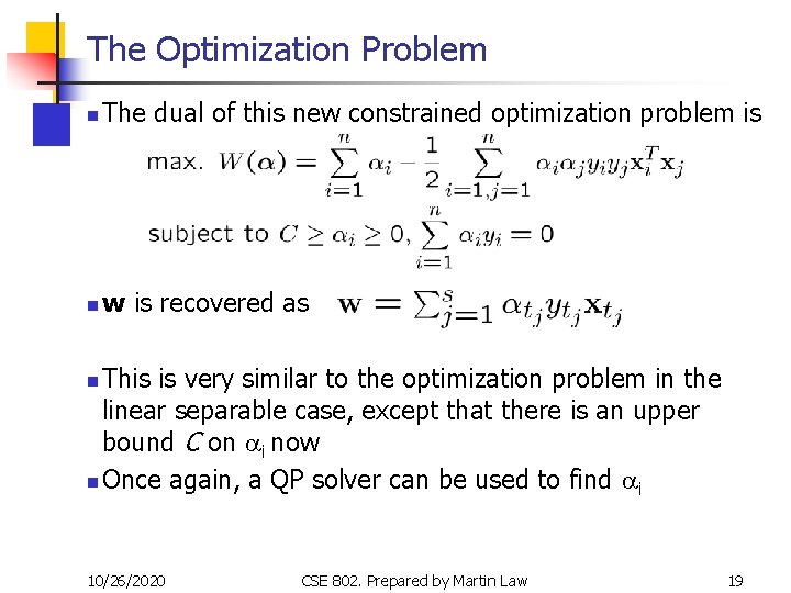
The Optimization Problem n The dual of this new constrained optimization problem is n w is recovered as This is very similar to the optimization problem in the linear separable case, except that there is an upper bound C on ai now n Once again, a QP solver can be used to find ai n 10/26/2020 CSE 802. Prepared by Martin Law 19

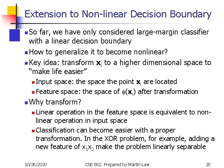
Extension to Non-linear Decision Boundary So far, we have only considered large-margin classifier with a linear decision boundary n How to generalize it to become nonlinear? n Key idea: transform xi to a higher dimensional space to “make life easier” n Input space: the space the point xi are located n Feature space: the space of f(xi) after transformation n n Why transform? Linear operation in the feature space is equivalent to nonlinear operation in input space n Classification can become easier with a proper transformation. In the XOR problem, for example, adding a new feature of x 1 x 2 make the problem linearly separable n 10/26/2020 CSE 802. Prepared by Martin Law 20

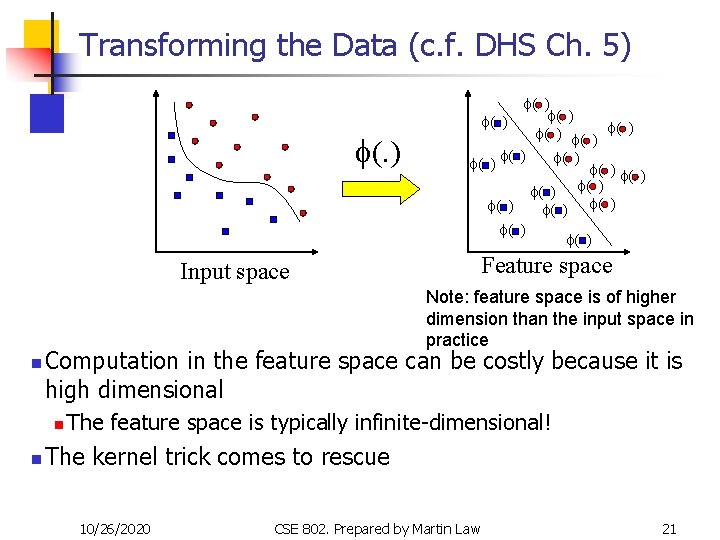
Transforming the Data (c. f. DHS Ch. 5) f( ) f( ) f( ) f( ) f( ) Feature space Input space Note: feature space is of higher dimension than the input space in practice n Computation in the feature space can be costly because it is high dimensional n n The feature space is typically infinite-dimensional! The kernel trick comes to rescue 10/26/2020 CSE 802. Prepared by Martin Law 21

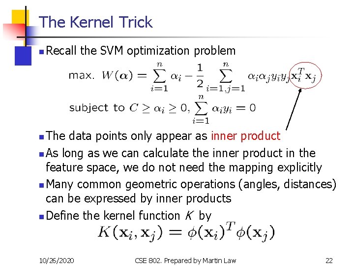
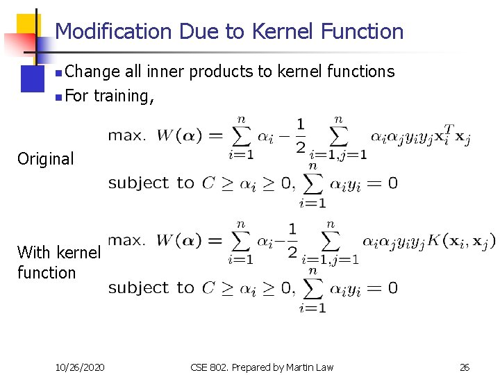
The Kernel Trick n Recall the SVM optimization problem The data points only appear as inner product n As long as we can calculate the inner product in the feature space, we do not need the mapping explicitly n Many common geometric operations (angles, distances) can be expressed by inner products n Define the kernel function K by n 10/26/2020 CSE 802. Prepared by Martin Law 22

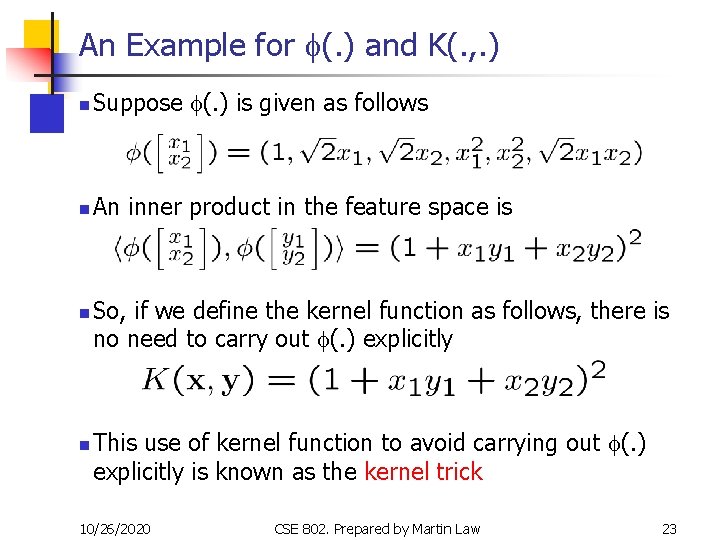
An Example for f(. ) and K(. , . ) n Suppose f(. ) is given as follows n An inner product in the feature space is n n So, if we define the kernel function as follows, there is no need to carry out f(. ) explicitly This use of kernel function to avoid carrying out f(. ) explicitly is known as the kernel trick 10/26/2020 CSE 802. Prepared by Martin Law 23

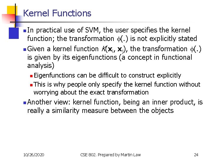
Kernel Functions In practical use of SVM, the user specifies the kernel function; the transformation f(. ) is not explicitly stated n Given a kernel function K(xi, xj), the transformation f(. ) is given by its eigenfunctions (a concept in functional analysis) n Eigenfunctions can be difficult to construct explicitly n This is why people only specify the kernel function without worrying about the exact transformation n n Another view: kernel function, being an inner product, is really a similarity measure between the objects 10/26/2020 CSE 802. Prepared by Martin Law 24

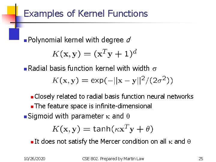
Examples of Kernel Functions n Polynomial kernel with degree d n Radial basis function kernel with width s Closely related to radial basis function neural networks n The feature space is infinite-dimensional n n Sigmoid with parameter k and q n It does not satisfy the Mercer condition on all k and q 10/26/2020 CSE 802. Prepared by Martin Law 25

Modification Due to Kernel Function Change all inner products to kernel functions n For training, n Original With kernel function 10/26/2020 CSE 802. Prepared by Martin Law 26

Modification Due to Kernel Function n For testing, the new data z is classified as class 1 if f ³ 0, and as class 2 if f <0 Original With kernel function 10/26/2020 CSE 802. Prepared by Martin Law 27

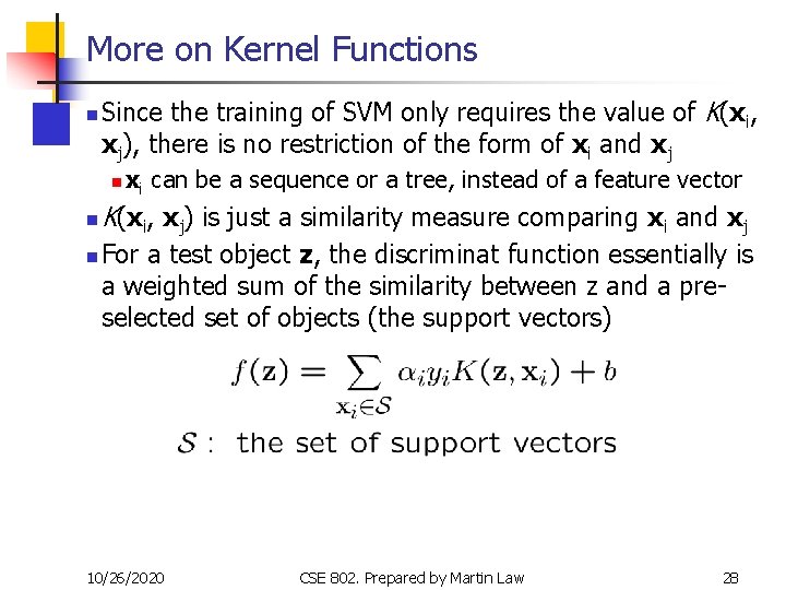
More on Kernel Functions n Since the training of SVM only requires the value of K(xi, xj), there is no restriction of the form of xi and xj n n n xi can be a sequence or a tree, instead of a feature vector K(xi, xj) is just a similarity measure comparing xi and xj For a test object z, the discriminat function essentially is a weighted sum of the similarity between z and a preselected set of objects (the support vectors) 10/26/2020 CSE 802. Prepared by Martin Law 28

More on Kernel Functions n Not all similarity measure can be used as kernel function, however The kernel function needs to satisfy the Mercer function, i. e. , the function is “positive-definite” n This implies that the n by n kernel matrix, in which the (i, j)th entry is the K(xi, xj), is always positive definite n This also means that the QP is convex and can be solved in polynomial time n 10/26/2020 CSE 802. Prepared by Martin Law 29

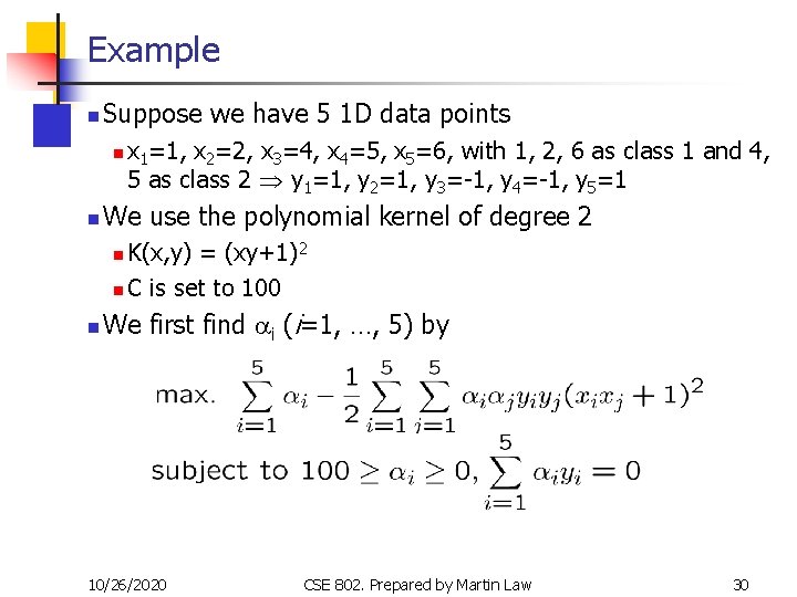
Example n Suppose we have 5 1 D data points n n x 1=1, x 2=2, x 3=4, x 4=5, x 5=6, with 1, 2, 6 as class 1 and 4, 5 as class 2 y 1=1, y 2=1, y 3=-1, y 4=-1, y 5=1 We use the polynomial kernel of degree 2 K(x, y) = (xy+1)2 n C is set to 100 n n We first find ai (i=1, …, 5) by 10/26/2020 CSE 802. Prepared by Martin Law 30

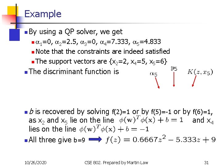
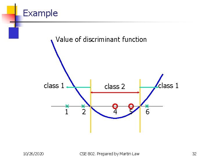
Example n By using a QP solver, we get a 1=0, a 2=2. 5, a 3=0, a 4=7. 333, a 5=4. 833 n Note that the constraints are indeed satisfied n The support vectors are {x 2=2, x 4=5, x 5=6} n n The discriminant function is n b is recovered by solving f(2)=1 as x 2 and x 5 lie on the line lies on the line n All three give b=9 10/26/2020 or by f(5)=-1 or by f(6)=1, and x 4 CSE 802. Prepared by Martin Law 31

Example Value of discriminant function class 1 1 10/26/2020 class 1 class 2 2 4 5 CSE 802. Prepared by Martin Law 6 32

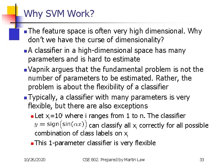
Why SVM Work? The feature space is often very high dimensional. Why don’t we have the curse of dimensionality? n A classifier in a high-dimensional space has many parameters and is hard to estimate n Vapnik argues that the fundamental problem is not the number of parameters to be estimated. Rather, the problem is about the flexibility of a classifier n Typically, a classifier with many parameters is very flexible, but there also exceptions n Let xi=10 i where i ranges from 1 to n. The classifier can classify all xi correctly for all possible combination of class labels on xi n This 1 -parameter classifier is very flexible n 10/26/2020 CSE 802. Prepared by Martin Law 33

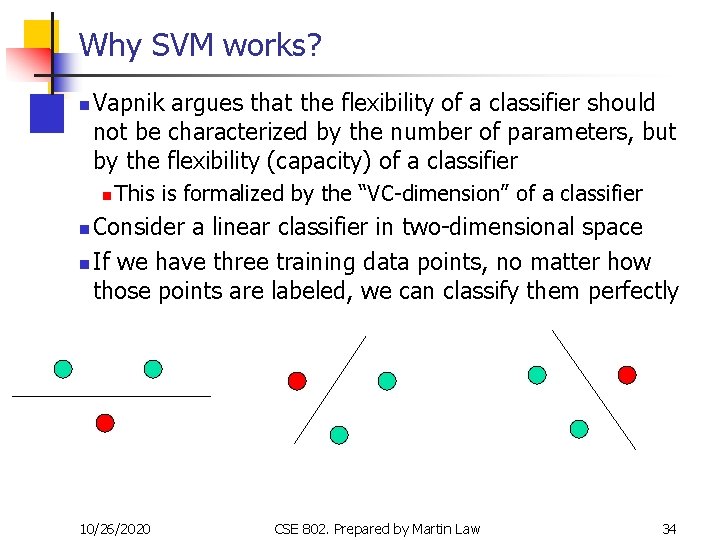
Why SVM works? n Vapnik argues that the flexibility of a classifier should not be characterized by the number of parameters, but by the flexibility (capacity) of a classifier n This is formalized by the “VC-dimension” of a classifier Consider a linear classifier in two-dimensional space n If we have three training data points, no matter how those points are labeled, we can classify them perfectly n 10/26/2020 CSE 802. Prepared by Martin Law 34

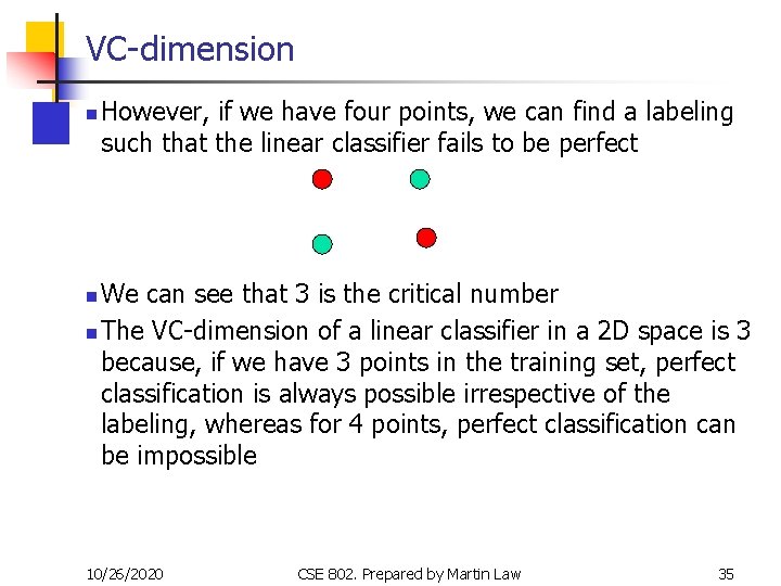
VC-dimension n However, if we have four points, we can find a labeling such that the linear classifier fails to be perfect We can see that 3 is the critical number n The VC-dimension of a linear classifier in a 2 D space is 3 because, if we have 3 points in the training set, perfect classification is always possible irrespective of the labeling, whereas for 4 points, perfect classification can be impossible n 10/26/2020 CSE 802. Prepared by Martin Law 35

VC-dimension The VC-dimension of the nearest neighbor classifier is infinity, because no matter how many points you have, you get perfect classification on training data n The higher the VC-dimension, the more flexible a classifier is n VC-dimension, however, is a theoretical concept; the VC -dimension of most classifiers, in practice, is difficult to be computed exactly n n Qualitatively, if we think a classifier is flexible, it probably has a high VC-dimension 10/26/2020 CSE 802. Prepared by Martin Law 36

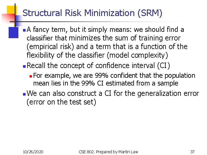
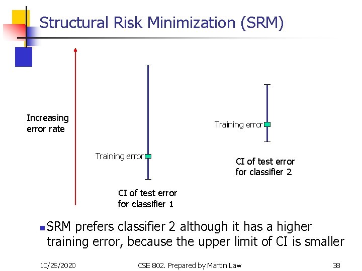
Structural Risk Minimization (SRM) A fancy term, but it simply means: we should find a classifier that minimizes the sum of training error (empirical risk) and a term that is a function of the flexibility of the classifier (model complexity) n Recall the concept of confidence interval (CI) n For example, we are 99% confident that the population mean lies in the 99% CI estimated from a sample n We can also construct a CI for the generalization error (error on the test set) n 10/26/2020 CSE 802. Prepared by Martin Law 37

Structural Risk Minimization (SRM) Increasing error rate Training error CI of test error for classifier 2 CI of test error for classifier 1 n SRM prefers classifier 2 although it has a higher training error, because the upper limit of CI is smaller 10/26/2020 CSE 802. Prepared by Martin Law 38

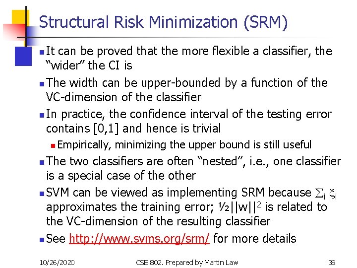
Structural Risk Minimization (SRM) It can be proved that the more flexible a classifier, the “wider” the CI is n The width can be upper-bounded by a function of the VC-dimension of the classifier n In practice, the confidence interval of the testing error contains [0, 1] and hence is trivial n n Empirically, minimizing the upper bound is still useful The two classifiers are often “nested”, i. e. , one classifier is a special case of the other n SVM can be viewed as implementing SRM because åi xi approximates the training error; ½||w||2 is related to the VC-dimension of the resulting classifier n See http: //www. svms. org/srm/ for more details n 10/26/2020 CSE 802. Prepared by Martin Law 39

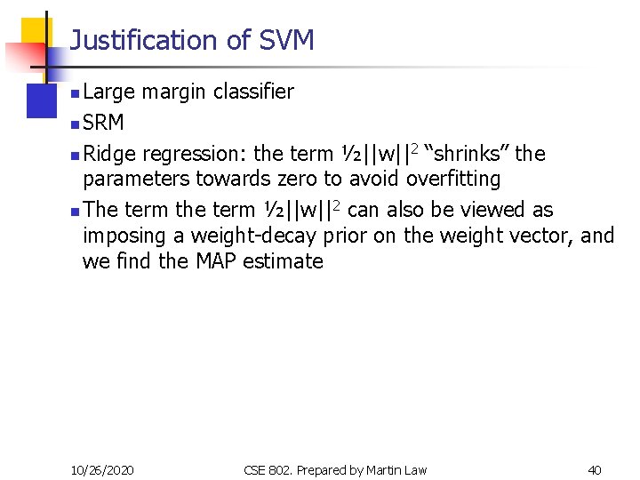
Justification of SVM Large margin classifier n SRM n Ridge regression: the term ½||w||2 “shrinks” the parameters towards zero to avoid overfitting n The term the term ½||w||2 can also be viewed as imposing a weight-decay prior on the weight vector, and we find the MAP estimate n 10/26/2020 CSE 802. Prepared by Martin Law 40

Choosing the Kernel Function Probably the most tricky part of using SVM. n The kernel function is important because it creates the kernel matrix, which summarizes all the data n Many principles have been proposed (diffusion kernel, Fisher kernel, string kernel, …) n There is even research to estimate the kernel matrix from available information n In practice, a low degree polynomial kernel or RBF kernel with a reasonable width is a good initial try n Note that SVM with RBF kernel is closely related to RBF neural networks, with the centers of the radial basis functions automatically chosen for SVM n 10/26/2020 CSE 802. Prepared by Martin Law 41

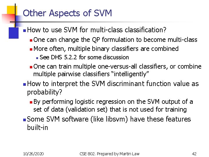
Other Aspects of SVM n How to use SVM for multi-classification? One can change the QP formulation to become multi-class n More often, multiple binary classifiers are combined n n One can train multiple one-versus-all classifiers, or combine multiple pairwise classifiers “intelligently” How to interpret the SVM discriminant function value as probability? n n See DHS 5. 2. 2 for some discussion By performing logistic regression on the SVM output of a set of data (validation set) that is not used for training Some SVM software (like libsvm) have these features built-in 10/26/2020 CSE 802. Prepared by Martin Law 42

Software A list of SVM implementation can be found at http: //www. kernel-machines. org/software. html n Some implementation (such as LIBSVM) can handle multi-classification n SVMLight is among one of the earliest implementation of SVM n Several Matlab toolboxes for SVM are also available n 10/26/2020 CSE 802. Prepared by Martin Law 43

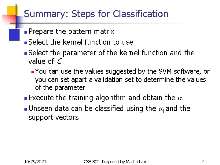
Summary: Steps for Classification Prepare the pattern matrix n Select the kernel function to use n Select the parameter of the kernel function and the value of C n n You can use the values suggested by the SVM software, or you can set apart a validation set to determine the values of the parameter Execute the training algorithm and obtain the ai n Unseen data can be classified using the ai and the support vectors n 10/26/2020 CSE 802. Prepared by Martin Law 44

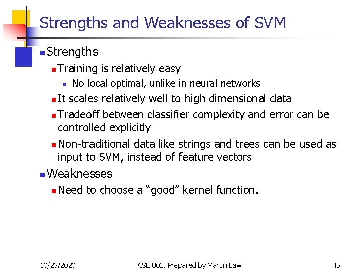
Strengths and Weaknesses of SVM n Strengths n Training is relatively easy n No local optimal, unlike in neural networks It scales relatively well to high dimensional data n Tradeoff between classifier complexity and error can be controlled explicitly n Non-traditional data like strings and trees can be used as input to SVM, instead of feature vectors n n Weaknesses n Need to choose a “good” kernel function. 10/26/2020 CSE 802. Prepared by Martin Law 45

Other Types of Kernel Methods A lesson learnt in SVM: a linear algorithm in the feature space is equivalent to a non-linear algorithm in the input space n Standard linear algorithms can be generalized to its nonlinear version by going to the feature space n n Kernel principal component analysis, kernel independent component analysis, kernel canonical correlation analysis, kernel k-means, 1 -class SVM are some examples 10/26/2020 CSE 802. Prepared by Martin Law 46

Conclusion SVM is a useful alternative to neural networks n Two key concepts of SVM: maximize the margin and the kernel trick n Many SVM implementations are available on the web for you to try on your data set! n 10/26/2020 CSE 802. Prepared by Martin Law 47

Resources http: //www. kernel-machines. org/ n http: //www. support-vector. net/icml-tutorial. pdf n http: //www. kernel-machines. org/papers/tutorialnips. gz n http: //www. clopinet. com/isabelle/Projects/SVM/applist. h tml n 10/26/2020 CSE 802. Prepared by Martin Law 48