SVM RVM Tipping 2003 Support Vector Machines Used

SVM & RVM Tipping (2003)

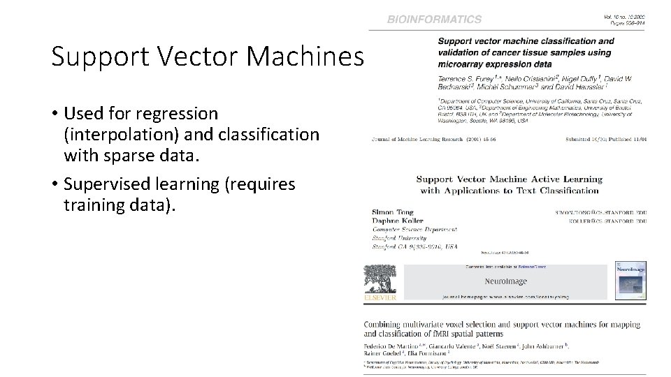
Support Vector Machines • Used for regression (interpolation) and classification with sparse data. • Supervised learning (requires training data).

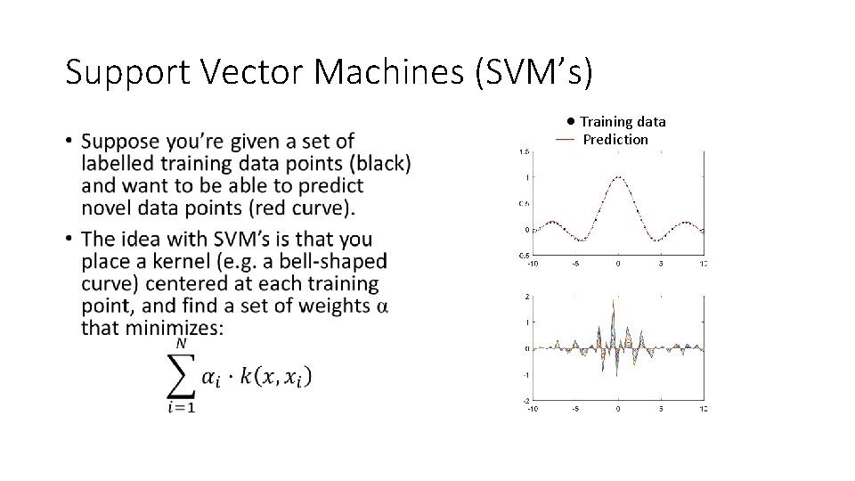
Support Vector Machines (SVM’s) • Training data Prediction

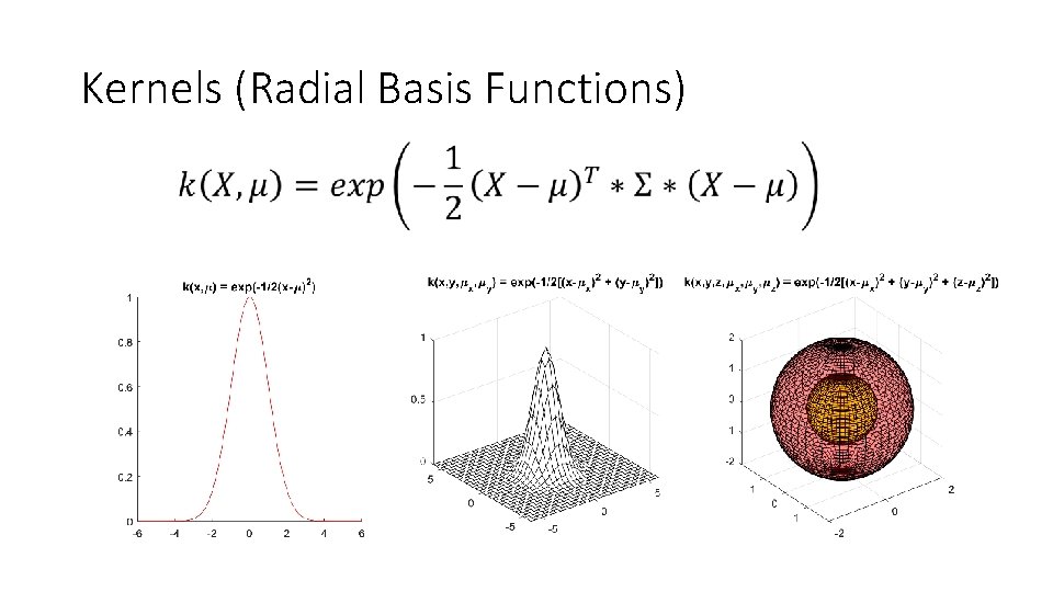
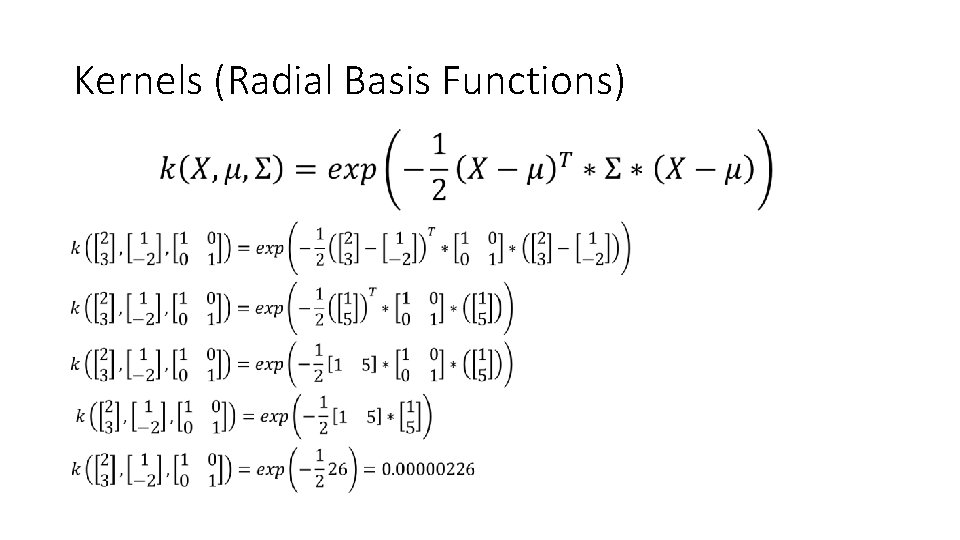
Kernels (Radial Basis Functions)

Kernels (Radial Basis Functions)

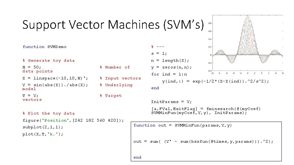
Support Vector Machines (SVM’s) function SVMDemo % --s = 1; % Generate toy data n = length(X); N = 50; data points % Number of y = zeros(n, n); X = linspace(-10, N)'; % Input vectors Y = sin(abs(X)). /abs(X); model % Underlying T = Y; vectors % Target subplot(2, 1, 1); y(ind, : ) = exp(-1/2*(X-X(ind)). ^2/s^2); end Init. Params = Y; [a, FVal, Exit. Flag] = fminsearch(@(my. Coef) SVMMin. Fun(my. Coef, Y, y), Init. Params); % Plot the toy data figure('Position', [242 182 560 420]); for ind = 1: n function out = SVMMin. Fun(params, Y, y) plot(X, T, 'k. '); out = sum( (Y' - sum(bsxfun(@times, y, params))). ^2); end

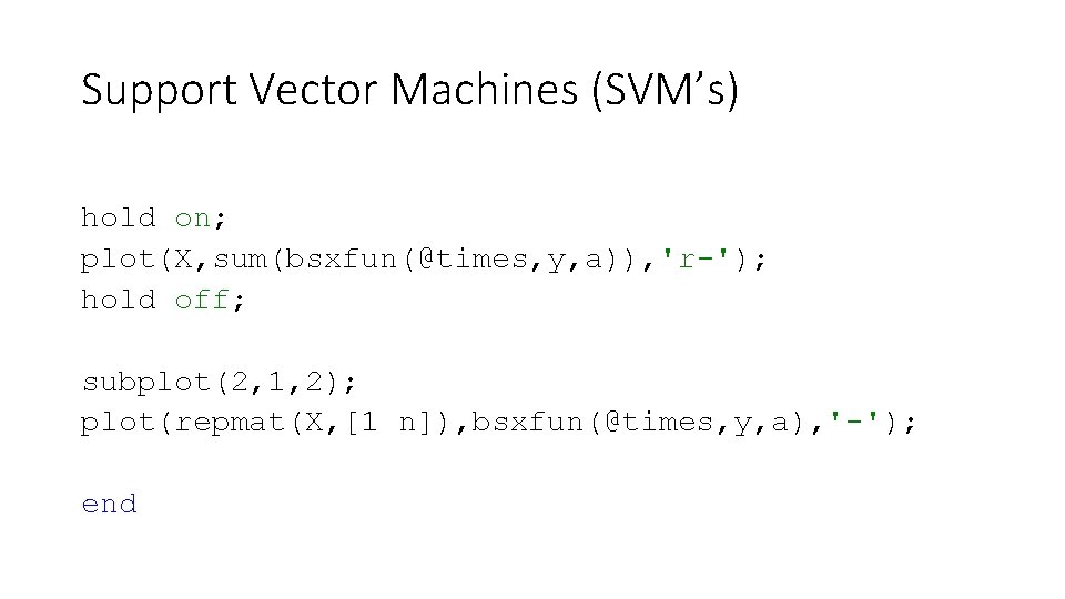
Support Vector Machines (SVM’s) hold on; plot(X, sum(bsxfun(@times, y, a)), 'r-'); hold off; subplot(2, 1, 2); plot(repmat(X, [1 n]), bsxfun(@times, y, a), '-'); end

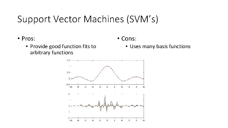
Support Vector Machines (SVM’s) • Pros: • Provide good function fits to arbitrary functions • Cons: • Uses many basis functions

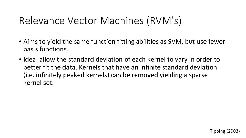
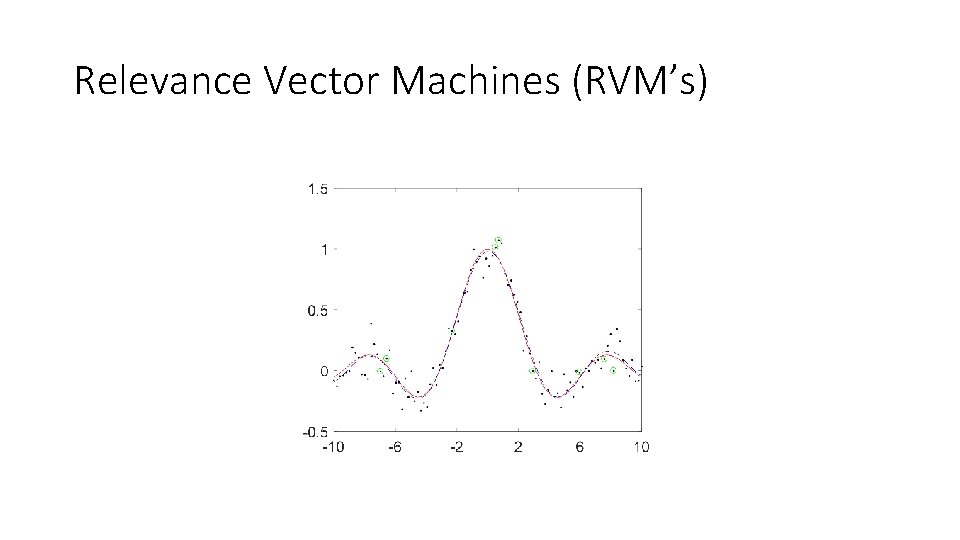
Relevance Vector Machines (RVM’s) • Aims to yield the same function fitting abilities as SVM, but use fewer basis functions. • Idea: allow the standard deviation of each kernel to vary in order to better fit the data. Kernels that have an infinite standard deviation (i. e. infinitely peaked kernels) can be removed yielding a sparse kernel set. Tipping (2003)

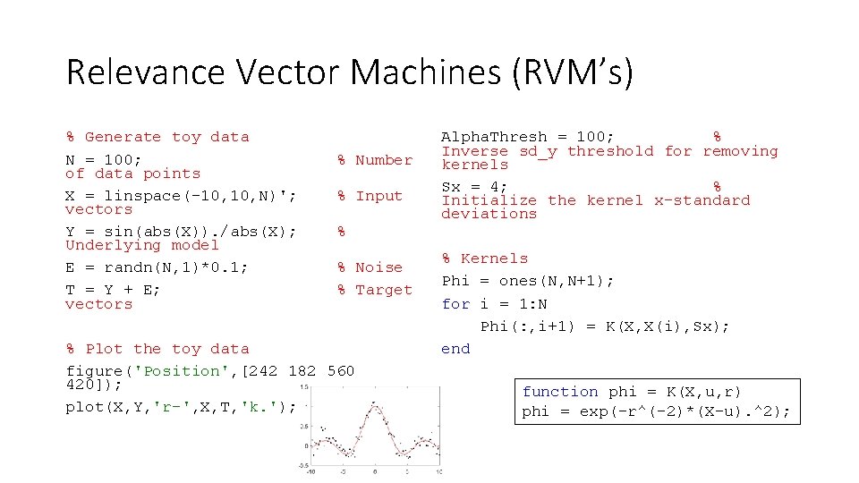
Relevance Vector Machines (RVM’s) % Generate toy data N = 100; of data points X = linspace(-10, N)'; vectors Y = sin(abs(X)). /abs(X); Underlying model E = randn(N, 1)*0. 1; T = Y + E; vectors % Number % Input % % Noise % Target % Plot the toy data figure('Position', [242 182 560 420]); plot(X, Y, 'r-', X, T, 'k. '); Alpha. Thresh = 100; % Inverse sd_y threshold for removing kernels Sx = 4; % Initialize the kernel x-standard deviations % Kernels Phi = ones(N, N+1); for i = 1: N Phi(: , i+1) = K(X, X(i), Sx); end function phi = K(X, u, r) phi = exp(-r^(-2)*(X-u). ^2);

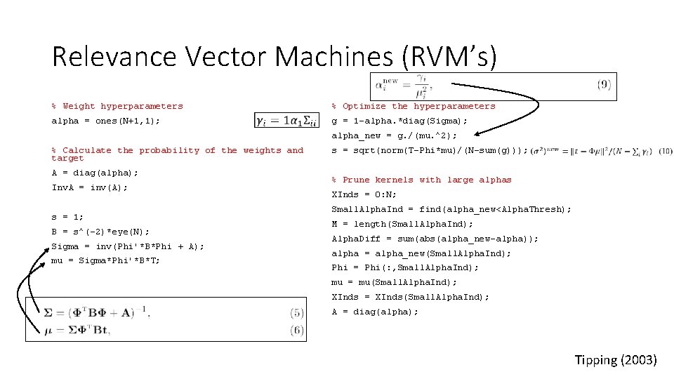
Relevance Vector Machines (RVM’s) % Weight hyperparameters alpha = ones(N+1, 1); % Optimize the hyperparameters g = 1 -alpha. *diag(Sigma); alpha_new = g. /(mu. ^2); % Calculate the probability of the weights and target A = diag(alpha); Inv. A = inv(A); s = 1; B = s^(-2)*eye(N); Sigma = inv(Phi'*B*Phi + A); mu = Sigma*Phi'*B*T; s = sqrt(norm(T-Phi*mu)/(N-sum(g))); % Prune kernels with large alphas XInds = 0: N; Small. Alpha. Ind = find(alpha_new<Alpha. Thresh); M = length(Small. Alpha. Ind); Alpha. Diff = sum(abs(alpha_new-alpha)); alpha = alpha_new(Small. Alpha. Ind); Phi = Phi(: , Small. Alpha. Ind); mu = mu(Small. Alpha. Ind); XInds = XInds(Small. Alpha. Ind); A = diag(alpha); Tipping (2003)

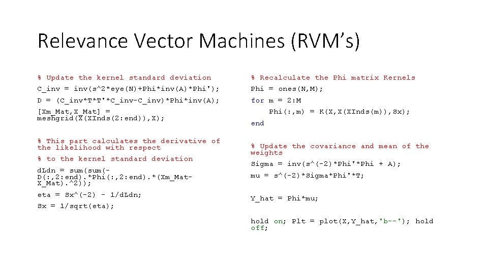
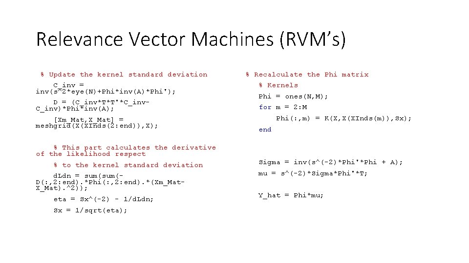
Relevance Vector Machines (RVM’s) % Update the kernel standard deviation % Recalculate the Phi matrix Kernels C_inv = inv(s^2*eye(N)+Phi*inv(A)*Phi'); Phi = ones(N, M); D = (C_inv*T*T'*C_inv-C_inv)*Phi*inv(A); for m = 2: M [Xm_Mat, X_Mat] = meshgrid(X(XInds(2: end)), X); % This part calculates the derivative of the likelihood with respect % to the kernel standard deviation d. Ldn = sum(D(: , 2: end). *Phi(: , 2: end). *(Xm_Mat. X_Mat). ^2)); eta = Sx^(-2) - 1/d. Ldn; Sx = 1/sqrt(eta); Phi(: , m) = K(X, X(XInds(m)), Sx); end % Update the covariance and mean of the weights Sigma = inv(s^(-2)*Phi'*Phi + A); mu = s^(-2)*Sigma*Phi'*T; Y_hat = Phi*mu; hold on; Plt = plot(X, Y_hat, 'b--'); hold off;

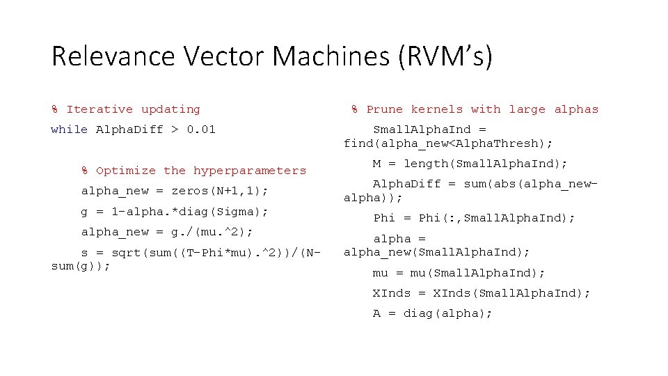
Relevance Vector Machines (RVM’s) % Iterative updating while Alpha. Diff > 0. 01 % Optimize the hyperparameters alpha_new = zeros(N+1, 1); g = 1 -alpha. *diag(Sigma); alpha_new = g. /(mu. ^2); s = sqrt(sum((T-Phi*mu). ^2))/(Nsum(g)); % Prune kernels with large alphas Small. Alpha. Ind = find(alpha_new<Alpha. Thresh); M = length(Small. Alpha. Ind); Alpha. Diff = sum(abs(alpha_newalpha)); Phi = Phi(: , Small. Alpha. Ind); alpha = alpha_new(Small. Alpha. Ind); mu = mu(Small. Alpha. Ind); XInds = XInds(Small. Alpha. Ind); A = diag(alpha);

Relevance Vector Machines (RVM’s) % Update the kernel standard deviation C_inv = inv(s^2*eye(N)+Phi*inv(A)*Phi'); D = (C_inv*T*T'*C_inv)*Phi*inv(A); [Xm_Mat, X_Mat] = meshgrid(X(XInds(2: end)), X); % Recalculate the Phi matrix % Kernels Phi = ones(N, M); for m = 2: M Phi(: , m) = K(X, X(XInds(m)), Sx); end % This part calculates the derivative of the likelihood respect % to the kernel standard deviation d. Ldn = sum(D(: , 2: end). *Phi(: , 2: end). *(Xm_Mat. X_Mat). ^2)); eta = Sx^(-2) - 1/d. Ldn; Sx = 1/sqrt(eta); Sigma = inv(s^(-2)*Phi'*Phi + A); mu = s^(-2)*Sigma*Phi'*T; Y_hat = Phi*mu;

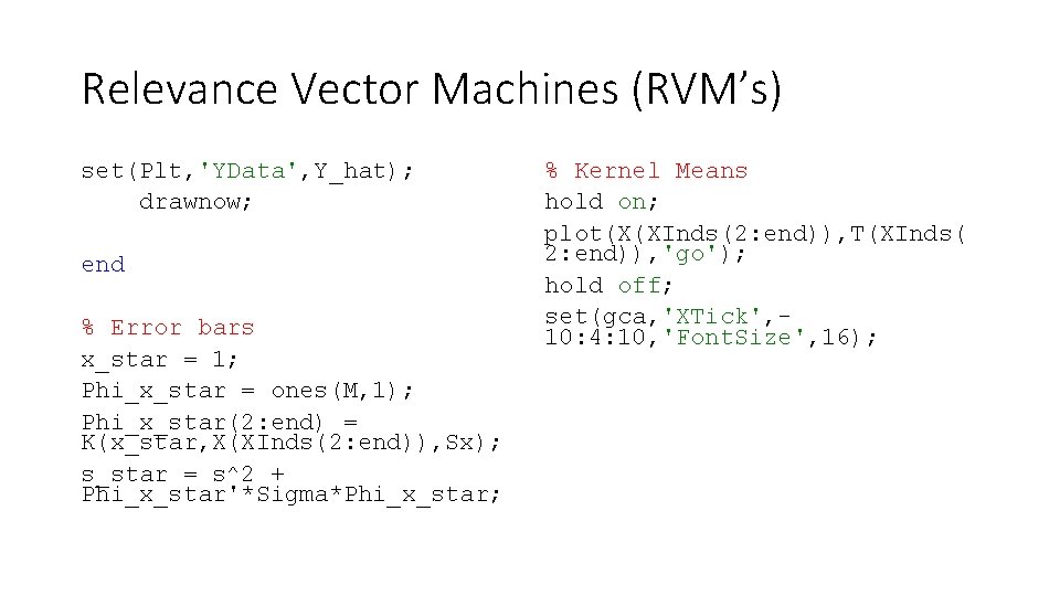
Relevance Vector Machines (RVM’s) set(Plt, 'YData', Y_hat); drawnow; end % Error bars x_star = 1; Phi_x_star = ones(M, 1); Phi_x_star(2: end) = K(x_star, X(XInds(2: end)), Sx); s_star = s^2 + Phi_x_star'*Sigma*Phi_x_star; % Kernel Means hold on; plot(X(XInds(2: end)), T(XInds( 2: end)), 'go'); hold off; set(gca, 'XTick', 10: 4: 10, 'Font. Size', 16);

Relevance Vector Machines (RVM’s)

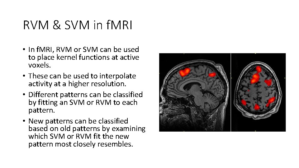
RVM & SVM in f. MRI • In f. MRI, RVM or SVM can be used to place kernel functions at active voxels. • These can be used to interpolate activity at a higher resolution. • Different patterns can be classified by fitting an SVM or RVM to each pattern. • New patterns can be classified based on old patterns by examining which SVM or RVM fit the new pattern most closely resembles.