An Introduction to Support Vector Machines Martin Law

An Introduction to Support Vector Machines Martin Law CSE 802. Prepared by Martin Law

Outline History of support vector machines (SVM) n Two classes, linearly separable n n What is a good decision boundary? Two classes, not linearly separable n How to make SVM non-linear: kernel trick n Demo of SVM n Epsilon support vector regression (e-SVR) n Conclusion n 5/19/2021 CSE 802. Prepared by Martin Law 2

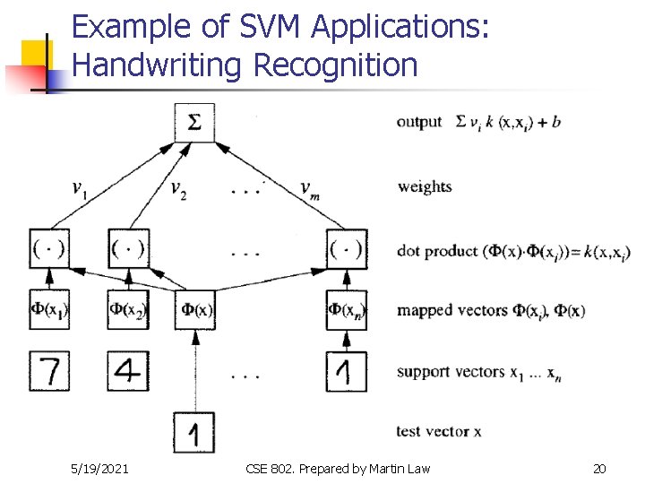
History of SVM is a classifier derived from statistical learning theory by Vapnik and Chervonenkis n SVM was first introduced in COLT-92 n SVM becomes famous when, using pixel maps as input, it gives accuracy comparable to sophisticated neural networks with elaborated features in a handwriting recognition task n Currently, SVM is closely related to: n n Kernel methods, large margin classifiers, reproducing kernel Hilbert space, Gaussian process 5/19/2021 CSE 802. Prepared by Martin Law 3

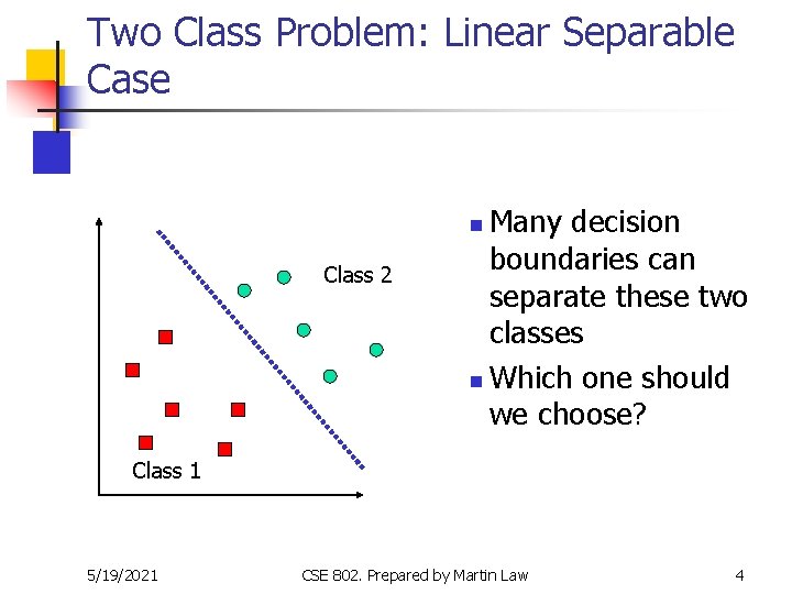
Two Class Problem: Linear Separable Case Many decision boundaries can separate these two classes n Which one should we choose? n Class 2 Class 1 5/19/2021 CSE 802. Prepared by Martin Law 4

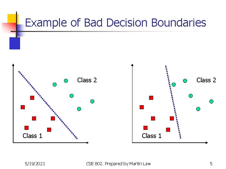
Example of Bad Decision Boundaries Class 2 Class 1 5/19/2021 Class 2 Class 1 CSE 802. Prepared by Martin Law 5

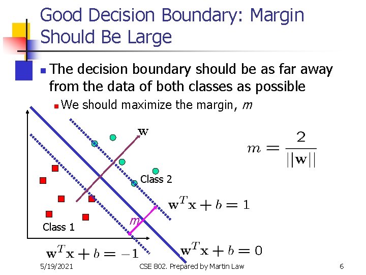
Good Decision Boundary: Margin Should Be Large n The decision boundary should be as far away from the data of both classes as possible n We should maximize the margin, m Class 2 Class 1 5/19/2021 m CSE 802. Prepared by Martin Law 6

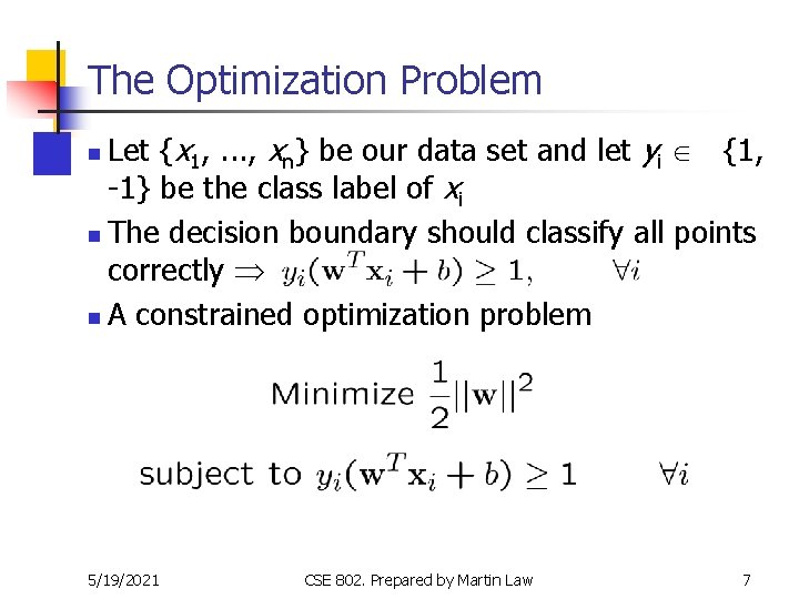
The Optimization Problem Let {x 1, . . . , xn} be our data set and let yi Î {1, -1} be the class label of xi n The decision boundary should classify all points correctly n A constrained optimization problem n 5/19/2021 CSE 802. Prepared by Martin Law 7

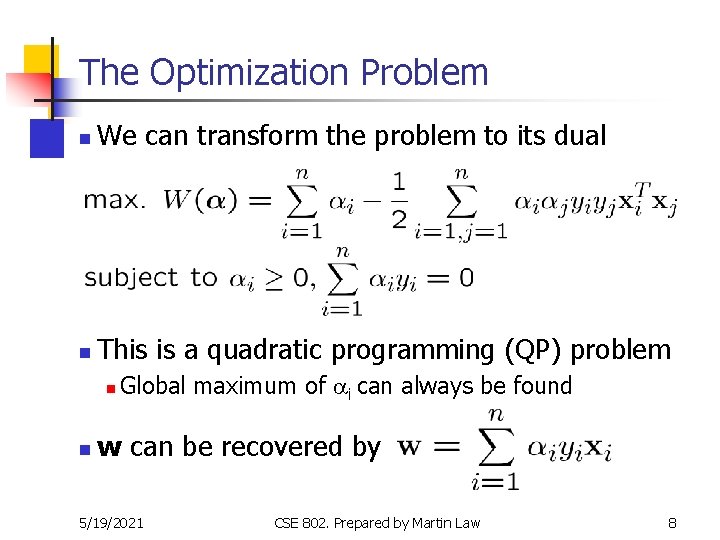
The Optimization Problem n We can transform the problem to its dual n This is a quadratic programming (QP) problem n n Global maximum of ai can always be found w can be recovered by 5/19/2021 CSE 802. Prepared by Martin Law 8

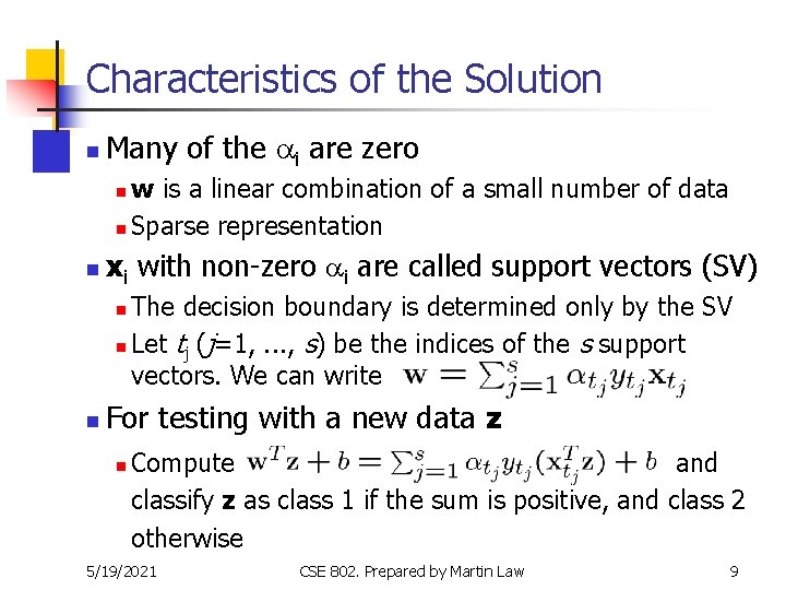
Characteristics of the Solution n Many of the ai are zero w is a linear combination of a small number of data n Sparse representation n n xi with non-zero ai are called support vectors (SV) The decision boundary is determined only by the SV n Let tj (j=1, . . . , s) be the indices of the s support vectors. We can write n n For testing with a new data z n Compute and classify z as class 1 if the sum is positive, and class 2 otherwise 5/19/2021 CSE 802. Prepared by Martin Law 9

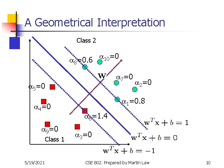
A Geometrical Interpretation Class 2 a 8=0. 6 a 10=0 a 7=0 a 5=0 a 4=0 a 9=0 Class 1 5/19/2021 a 2=0 a 1=0. 8 a 6=1. 4 a 3=0 CSE 802. Prepared by Martin Law 10

Some Notes n There are theoretical upper bounds on the error on unseen data for SVM The larger the margin, the smaller the bound n The smaller the number of SV, the smaller the bound n n Note that in both training and testing, the data are referenced only as inner product, x. Ty n This is important for generalizing to the non-linear case 5/19/2021 CSE 802. Prepared by Martin Law 11

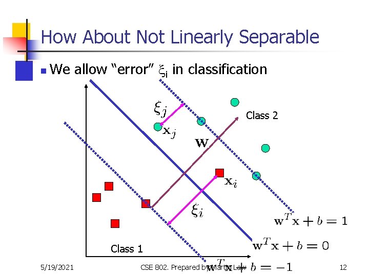
How About Not Linearly Separable n We allow “error” xi in classification Class 2 Class 1 5/19/2021 CSE 802. Prepared by Martin Law 12

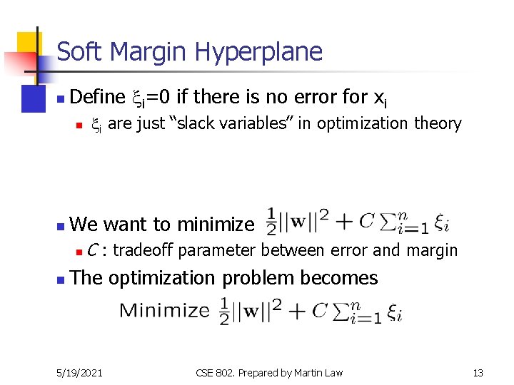
Soft Margin Hyperplane n Define xi=0 if there is no error for xi n n We want to minimize n n xi are just “slack variables” in optimization theory C : tradeoff parameter between error and margin The optimization problem becomes 5/19/2021 CSE 802. Prepared by Martin Law 13

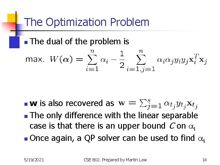
The Optimization Problem n The dual of the problem is w is also recovered as n The only difference with the linear separable case is that there is an upper bound C on ai n Once again, a QP solver can be used to find ai n 5/19/2021 CSE 802. Prepared by Martin Law 14

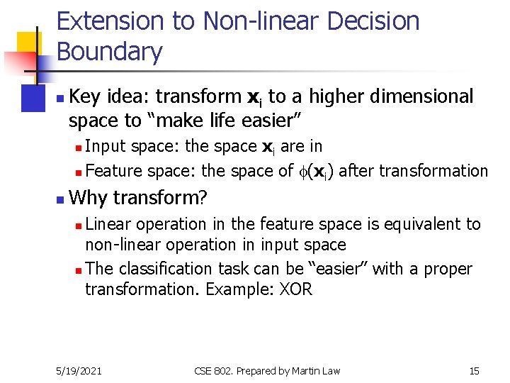
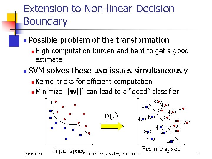
Extension to Non-linear Decision Boundary n Key idea: transform xi to a higher dimensional space to “make life easier” Input space: the space xi are in n Feature space: the space of f(xi) after transformation n n Why transform? Linear operation in the feature space is equivalent to non-linear operation in input space n The classification task can be “easier” with a proper transformation. Example: XOR n 5/19/2021 CSE 802. Prepared by Martin Law 15

Extension to Non-linear Decision Boundary n Possible problem of the transformation n n High computation burden and hard to get a good estimate SVM solves these two issues simultaneously Kernel tricks for efficient computation 2 n Minimize ||w|| can lead to a “good” classifier n f(. ) 5/19/2021 f( ) f( ) f( ) f( ) f( ) Feature space Input space CSE 802. Prepared by Martin Law 16

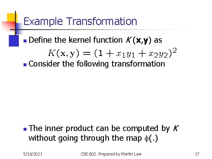
Example Transformation n Define the kernel function K (x, y) as n Consider the following transformation n The inner product can be computed by K without going through the map f(. ) 5/19/2021 CSE 802. Prepared by Martin Law 17

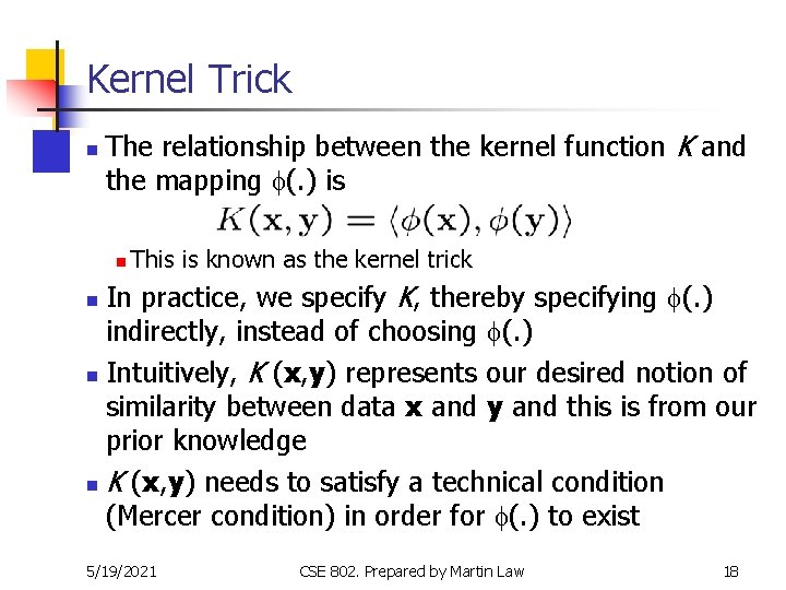
Kernel Trick n The relationship between the kernel function K and the mapping f(. ) is n This is known as the kernel trick In practice, we specify K, thereby specifying f(. ) indirectly, instead of choosing f(. ) n Intuitively, K (x, y) represents our desired notion of similarity between data x and y and this is from our prior knowledge n K (x, y) needs to satisfy a technical condition (Mercer condition) in order for f(. ) to exist n 5/19/2021 CSE 802. Prepared by Martin Law 18

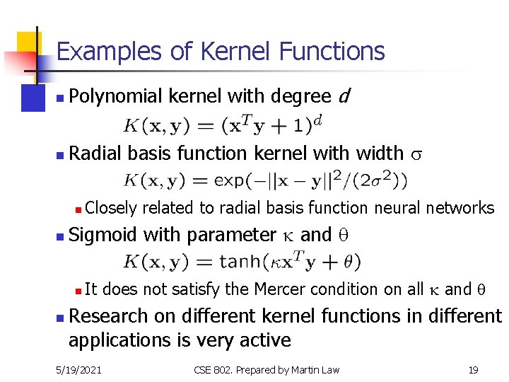
Examples of Kernel Functions n Polynomial kernel with degree d n Radial basis function kernel with width s n n Sigmoid with parameter k and q n n Closely related to radial basis function neural networks It does not satisfy the Mercer condition on all k and q Research on different kernel functions in different applications is very active 5/19/2021 CSE 802. Prepared by Martin Law 19

Example of SVM Applications: Handwriting Recognition 5/19/2021 CSE 802. Prepared by Martin Law 20

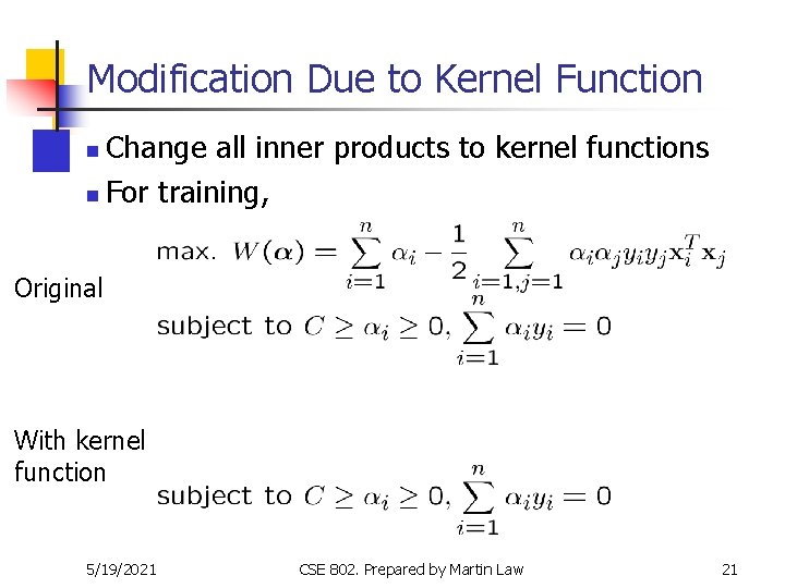
Modification Due to Kernel Function Change all inner products to kernel functions n For training, n Original With kernel function 5/19/2021 CSE 802. Prepared by Martin Law 21

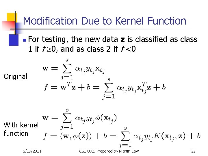
Modification Due to Kernel Function n For testing, the new data z is classified as class 1 if f ³ 0, and as class 2 if f <0 Original With kernel function 5/19/2021 CSE 802. Prepared by Martin Law 22

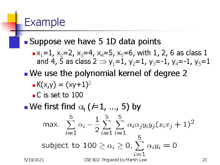
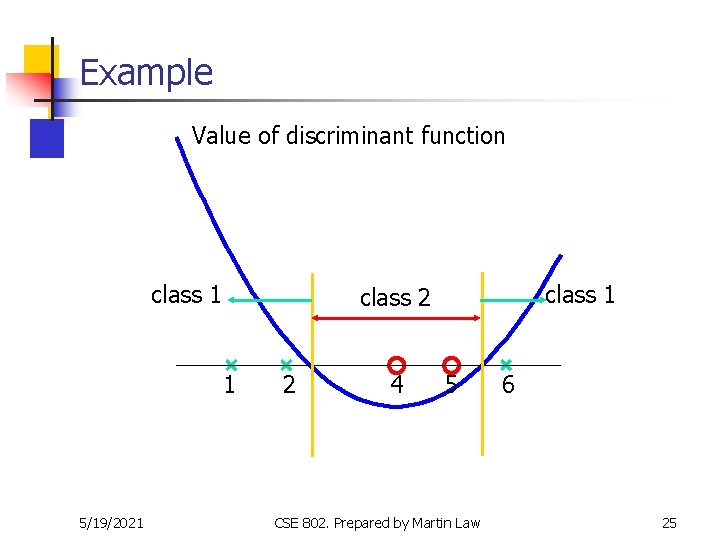
Example n Suppose we have 5 1 D data points n n x 1=1, x 2=2, x 3=4, x 4=5, x 5=6, with 1, 2, 6 as class 1 and 4, 5 as class 2 y 1=1, y 2=1, y 3=-1, y 4=-1, y 5=1 We use the polynomial kernel of degree 2 K(x, y) = (xy+1)2 n C is set to 100 n n We first find ai (i=1, …, 5) by 5/19/2021 CSE 802. Prepared by Martin Law 23

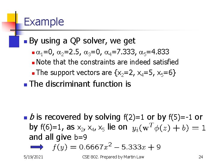
Example n By using a QP solver, we get a 1=0, a 2=2. 5, a 3=0, a 4=7. 333, a 5=4. 833 n Note that the constraints are indeed satisfied n The support vectors are {x 2=2, x 4=5, x 5=6} n n The discriminant function is n b is recovered by solving f(2)=1 or by f(5)=-1 or by f(6)=1, as x 2, x 4, x 5 lie on and all give b=9 5/19/2021 CSE 802. Prepared by Martin Law 24

Example Value of discriminant function class 1 1 5/19/2021 class 2 2 4 5 CSE 802. Prepared by Martin Law 6 25

Multi-class Classification SVM is basically a two-classifier n One can change the QP formulation to allow multi-classification n More commonly, the data set is divided into two parts “intelligently” in different ways and a separate SVM is trained for each way of division n Multi-classification is done by combining the output of all the SVM classifiers n Majority rule n Error correcting code n Directed acyclic graph n 5/19/2021 CSE 802. Prepared by Martin Law 26

Software A list of SVM implementation can be found at http: //www. kernel-machines. org/software. html n Some implementation (such as LIBSVM) can handle multi-classification n SVMLight is among one of the earliest implementation of SVM n Several Matlab toolboxes for SVM are also available n 5/19/2021 CSE 802. Prepared by Martin Law 27

Summary: Steps for Classification Prepare the pattern matrix n Select the kernel function to use n Select the parameter of the kernel function and the value of C n n You can use the values suggested by the SVM software, or you can set apart a validation set to determine the values of the parameter Execute the training algorithm and obtain the ai n Unseen data can be classified using the ai and the support vectors n 5/19/2021 CSE 802. Prepared by Martin Law 28

Demonstration n Iris data set n Class 1 and class 3 are “merged” in this demo 5/19/2021 CSE 802. Prepared by Martin Law 29

Strengths and Weaknesses of SVM n Strengths n Training is relatively easy n No local optimal, unlike in neural networks It scales relatively well to high dimensional data n Tradeoff between classifier complexity and error can be controlled explicitly n Non-traditional data like strings and trees can be used as input to SVM, instead of feature vectors n n Weaknesses n Need a “good” kernel function 5/19/2021 CSE 802. Prepared by Martin Law 30

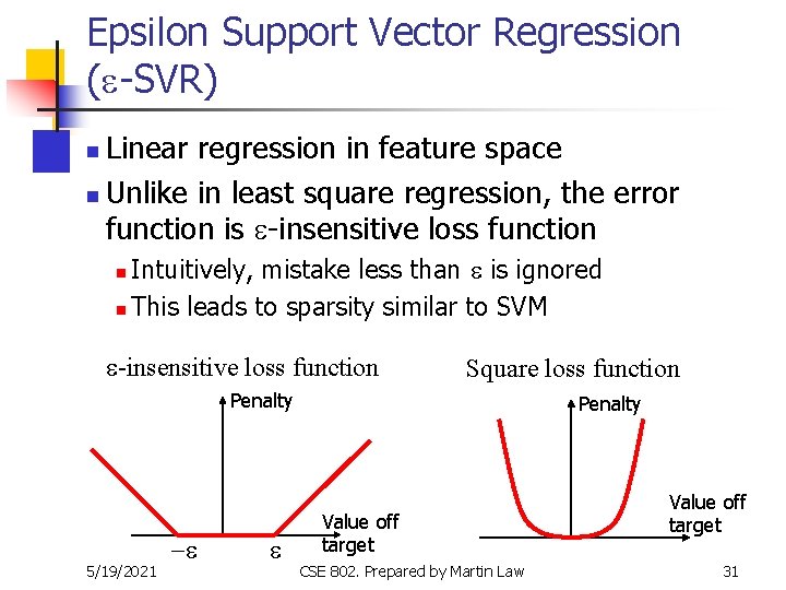
Epsilon Support Vector Regression (e-SVR) Linear regression in feature space n Unlike in least square regression, the error function is e-insensitive loss function n Intuitively, mistake less than e is ignored n This leads to sparsity similar to SVM n e-insensitive loss function Square loss function Penalty 5/19/2021 -e e Penalty Value off target CSE 802. Prepared by Martin Law Value off target 31

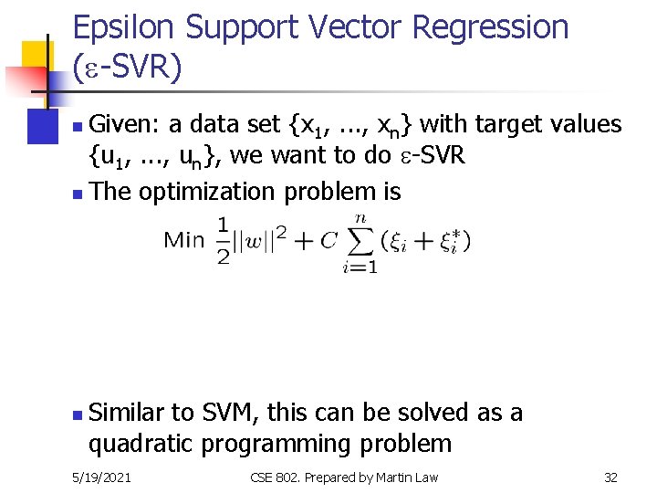
Epsilon Support Vector Regression (e-SVR) Given: a data set {x 1, . . . , xn} with target values {u 1, . . . , un}, we want to do e-SVR n The optimization problem is n n Similar to SVM, this can be solved as a quadratic programming problem 5/19/2021 CSE 802. Prepared by Martin Law 32

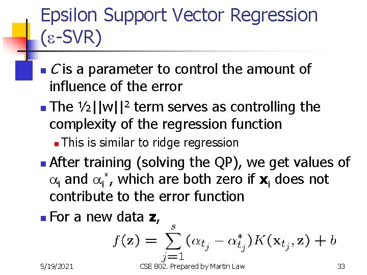
Epsilon Support Vector Regression (e-SVR) n C is a parameter to control the amount of influence of the error n The ½||w||2 term serves as controlling the complexity of the regression function n This is similar to ridge regression After training (solving the QP), we get values of ai and ai*, which are both zero if xi does not contribute to the error function n For a new data z, n 5/19/2021 CSE 802. Prepared by Martin Law 33

Other Types of Kernel Methods A lesson learnt in SVM: a linear algorithm in the feature space is equivalent to a non-linear algorithm in the input space n Classic linear algorithms can be generalized to its non-linear version by going to the feature space n n Kernel principal component analysis, kernel independent component analysis, kernel canonical correlation analysis, kernel k-means, 1 -class SVM are some examples 5/19/2021 CSE 802. Prepared by Martin Law 34

Conclusion SVM is a useful alternative to neural networks n Two key concepts of SVM: maximize the margin and the kernel trick n Many active research is taking place on areas related to SVM n Many SVM implementations are available on the web for you to try on your data set! n 5/19/2021 CSE 802. Prepared by Martin Law 35

Resources http: //www. kernel-machines. org/ n http: //www. support-vector. net/icml-tutorial. pdf n http: //www. kernel-machines. org/papers/tutorial -nips. gz n http: //www. clopinet. com/isabelle/Projects/SVM/ applist. html n 5/19/2021 CSE 802. Prepared by Martin Law 36