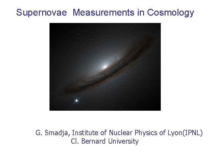
Supernovae Measurements in Cosmology G Smadja Institute of

Supernovae Measurements in Cosmology G. Smadja, Institute of Nuclear Physics of Lyon(IPNL) Cl. Bernard University

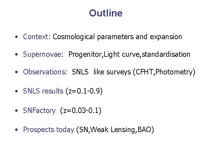
Outline • Context: Cosmological parameters and expansion • Supernovae: Progenitor, Light curve, standardisation • Observations: SNLS like surveys (CFHT, Photometry) • SNLS results (z=0. 1 -0. 9) • SNFactory (z=0. 03 -0. 1) • Prospects today (SN, Weak Lensing, BAO)

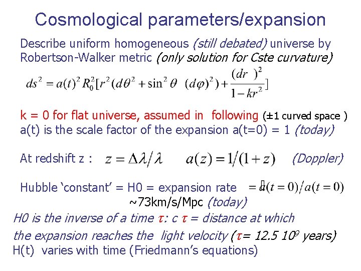
Cosmological parameters/expansion Describe uniform homogeneous (still debated) universe by Robertson-Walker metric (only solution for Cste curvature) k = 0 for flat universe, assumed in following (± 1 curved space ) a(t) is the scale factor of the expansion a(t=0) = 1 (today) At redshift z : (Doppler) Hubble ‘constant’ = H 0 = expansion rate ~73 km/s/Mpc (today) H 0 is the inverse of a time t: c t = distance at which the expansion reaches the light velocity (t= 12. 5 109 years) H(t) varies with time (Friedmann’s equations)

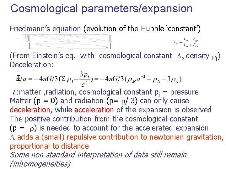
Cosmological parameters/expansion Friedmann’s equation (evolution of the Hubble ‘constant’) (From Einstein’s eq. with cosmological constant L, density ri) Deceleration: i : matter , radiation, cosmological constant pi = pressure Matter (p = 0) and radiation (p= r/ 3) can only cause deceleration, while acceleration of the expansion is observed The positive contribution from the cosmological constant (p = -r) is needed to account for the accelerated expansion L adds a (small) repulsive contribution to newtonian gravitation, proportional to distance Some non standard interpretation of data still remain (inhomogeneities)

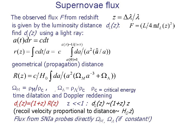
Supernovae flux The observed flux F from redshift is given by the luminosity distance d. L(z): find d. L(z) using a light ray: geometrical (propagation) distance WM = r. M/rc , , WL = r. L/rc rc = critical energy time dilatation and Doppler reddening d. L(z)=(1+z) R(z) z <<1 : d. L(z) ~(1+z) z (recoil velocity proportional to distance~ H 0 z) Flux from SNIa probes directly WM , WL (if constant!)

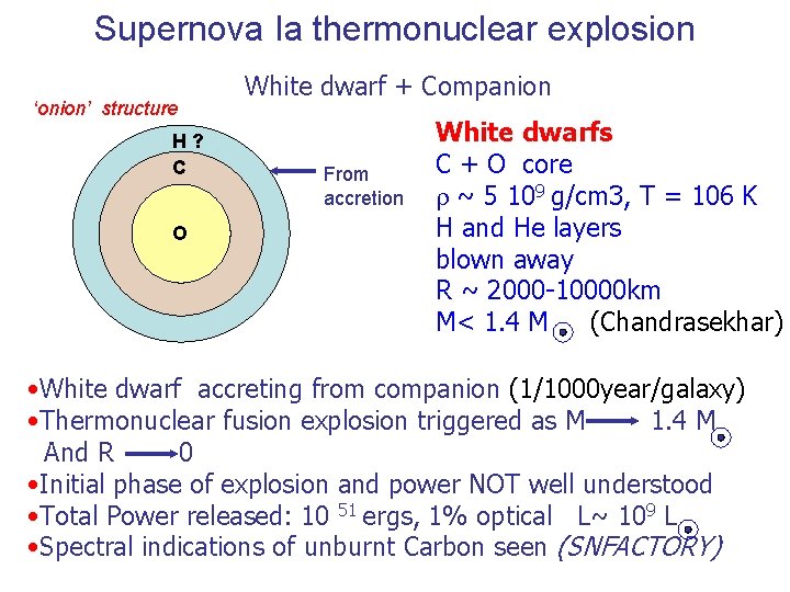
Supernova Ia thermonuclear explosion ‘onion’ structure H? C O White dwarf + Companion From accretion White dwarfs C + O core r ~ 5 109 g/cm 3, T = 106 K H and He layers blown away R ~ 2000 -10000 km M< 1. 4 M (Chandrasekhar) • White dwarf accreting from companion (1/1000 year/galaxy) • Thermonuclear fusion explosion triggered as M 1. 4 M And R 0 • Initial phase of explosion and power NOT well understood • Total Power released: 10 51 ergs, 1% optical L~ 109 L • Spectral indications of unburnt Carbon seen (SNFACTORY)

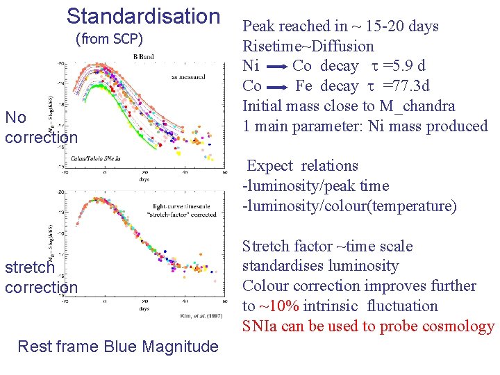
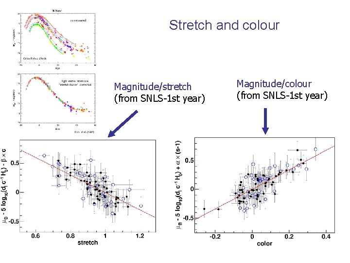
Standardisation (from SCP) No correction Peak reached in ~ 15 -20 days Risetime~Diffusion Ni Co decay t =5. 9 d Co Fe decay t =77. 3 d Initial mass close to M_chandra 1 main parameter: Ni mass produced Expect relations -luminosity/peak time -luminosity/colour(temperature) stretch correction Rest frame Blue Magnitude Stretch factor ~time scale standardises luminosity Colour correction improves further to ~10% intrinsic fluctuation SNIa can be used to probe cosmology

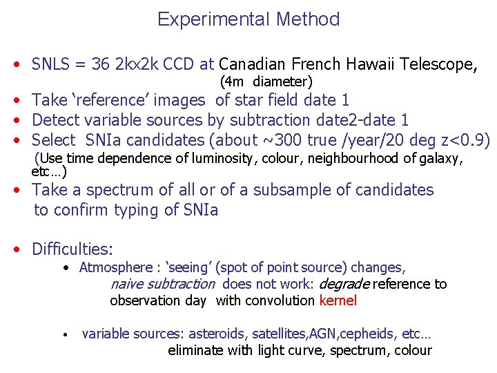
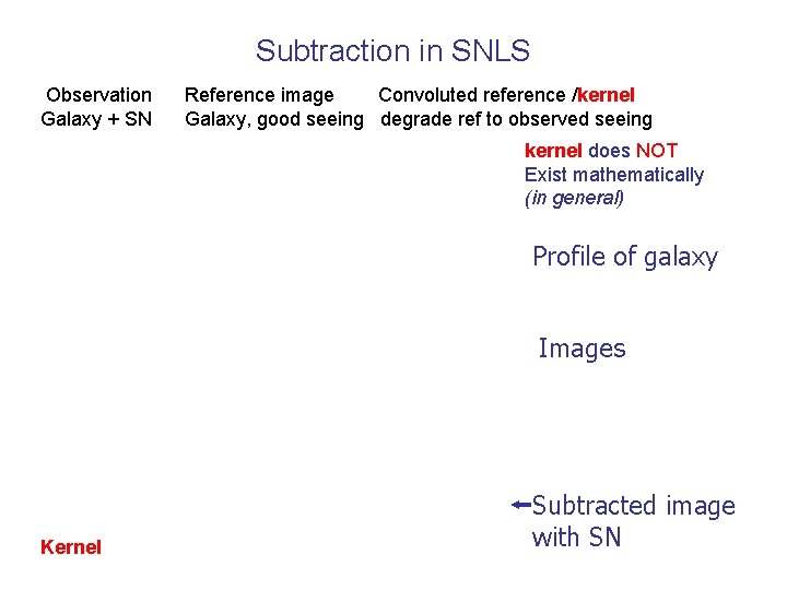
Experimental Method • SNLS = 36 2 kx 2 k CCD at Canadian French Hawaii Telescope, (4 m diameter) • Take ‘reference’ images of star field date 1 • Detect variable sources by subtraction date 2 -date 1 • Select SNIa candidates (about ~300 true /year/20 deg z<0. 9) (Use time dependence of luminosity, colour, neighbourhood of galaxy, etc…) • Take a spectrum of all or of a subsample of candidates to confirm typing of SNIa • Difficulties: • Atmosphere : ‘seeing’ (spot of point source) changes, naive subtraction does not work: degrade reference to observation day with convolution kernel • variable sources: asteroids, satellites, AGN, cepheids, etc… eliminate with light curve, spectrum, colour

Subtraction in SNLS Observation Galaxy + SN Reference image Convoluted reference /kernel Galaxy, good seeing degrade ref to observed seeing kernel does NOT Exist mathematically (in general) Profile of galaxy Images Kernel Subtracted image with SN

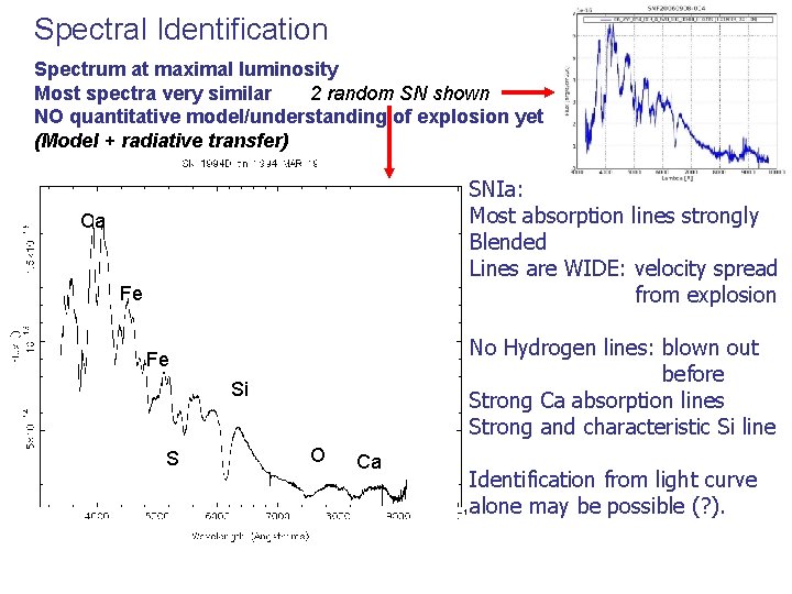
Spectral Identification Spectrum at maximal luminosity Most spectra very similar 2 random SN shown NO quantitative model/understanding of explosion yet (Model + radiative transfer) SNIa: Most absorption lines strongly Blended Lines are WIDE: velocity spread from explosion No Hydrogen lines: blown out before Strong Ca absorption lines Strong and characteristic Si line Ca Fe Fe Si S O Ca Identification from light curve alone may be possible (? ).

Stretch and colour Magnitude/stretch (from SNLS-1 st year) Magnitude/colour (from SNLS-1 st year)

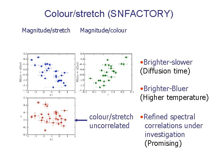
Colour/stretch (SNFACTORY) Magnitude/stretch Magnitude/colour • Brighter-slower (Diffusion time) • Brighter-Bluer (Higher temperature) colour/stretch • Refined spectral uncorrelated correlations under investigation (Promising)

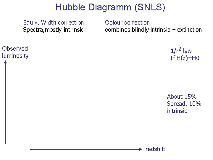
Hubble Diagramm (SNLS) Equiv. Width correction Spectra, mostly intrinsic Colour correction combines blindly intrinsic + extinction 1/r 2 law If H(z)=H 0 Observed luminosity About 15% Spread, 10% intrinsic redshift

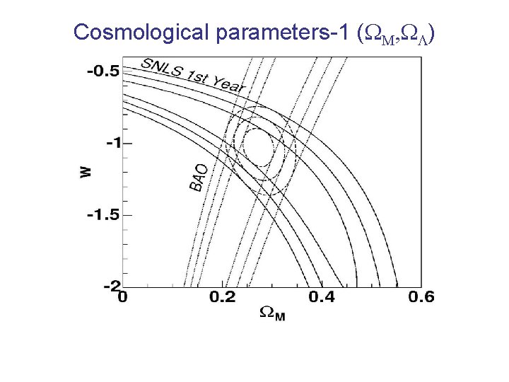
Cosmological parameters-1 (WM, WL)

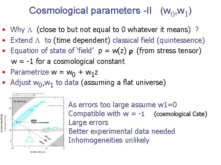
Cosmological parameters -II (w 0, w 1) • Why L (close to but not equal to 0 whatever it means) ? • Extend L to (time dependent) classical field (quintessence) • Equation of state of ‘field’ p = w(z) r (from stress tensor) w = -1 for a cosmological constant • Parametrize w = w 0 + w 1 z • Adjust w 0, w 1 to data (assuming a flat universe) As errors too large assume w 1=0 Compatible with w = -1 (cosmological Cste) Large errors Better experimental data needed Inhomogeneities unlikely

Improving data on Eq. of state • Dark energy constant L or field? Constant simpler, field has strange features, but … • Data must be improved • Decrease systematics (10%) (Go to space) • Extend range/lever arm • Up to z=1. 7 (Go to space + NIR detectors) • Down to 0. 03<z<0. 1 (more statistics) • Use other techniques: Weak Lensing, BAO • SNFactory adresses the low z issue • Spectrophotometry as a tool for • Understanding of SN explosions • Tests of evolution from near (low z) to distant (high z) • Create spectral templates at all phases for light curves

The SNFACTORY collaboration • Cover the range 0. 03<z<0. 1 (Hubble flow + exposure time) • Measure spectra at all dates : improve light curve measurements In photometric filters (time dependent create templates) • Measure the total flux: no slit spectroscopy Integral Field Spectrograph • SNFACTORY Collaboration: LBNL (Berkeley)Aldering, Perlmutter Yale C. Baltay CRAL(Lyon) Pecontal IPNL(Lyon) G. S. , Y. Copin LPNHE(Paris) R. Pain • Search at Quest 1 m, Palomar, Yale CCD Camera (US teams) • Spectroscopy at UH 2 m with IFS SNIFS from Lyon

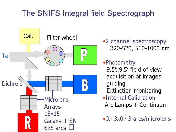
The SNIFS Integral field Spectrograph Cal. Filter wheel Tel Dichroic Microlens Arrays 15 x 15 Galaxy + SN 6 x 6 arcs • 2 channel spectroscopy 320 -520, 510 -1000 nm • Photometry 9. 5’x 9. 5’ field of view acquisition of images guiding Extinction monitoring • Internal Calibration Arc Lamps + Continuum • 0. 43 x 0. 43 arcs/microlens

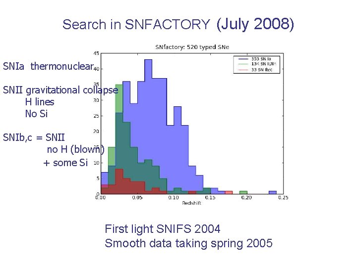
Search in SNFACTORY (July 2008) SNIa thermonuclear SNII gravitational collapse H lines No Si SNIb, c = SNII no H (blown) + some Si First light SNIFS 2004 Smooth data taking spring 2005

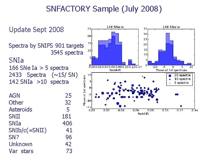
SNFACTORY Sample (July 2008) Update Sept 2008 Spectra by SNIFS 901 targets 3545 spectra SNIa 166 SNe Ia > 5 spectra 2433 Spectra (~15/ SN) 142 SNIa >10 spectra AGN 25 Other 32 Asteroids 5 SNII 181 SNIa 406 SNIb/c(=SNII) 41 SN? 96 Unknown 42 Var stars 73

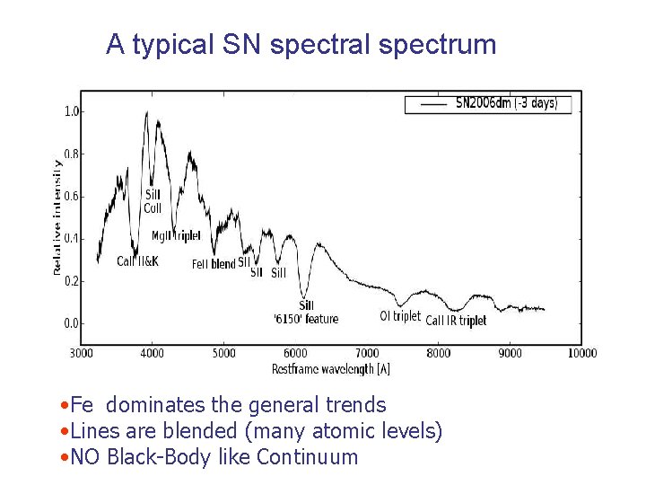
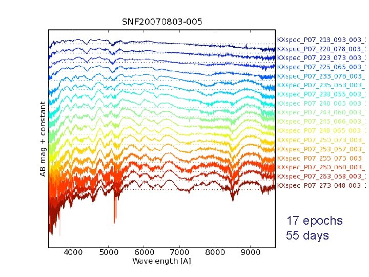
A typical SN spectral spectrum • Fe dominates the general trends • Lines are blended (many atomic levels) • NO Black-Body like Continuum

A Time sequence 17 epochs 55 days

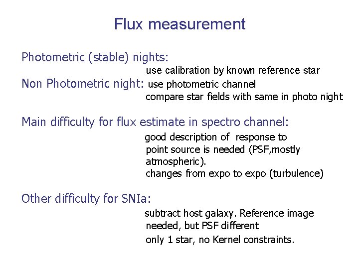
Flux measurement Photometric (stable) nights: use calibration by known reference star Non Photometric night: use photometric channel compare star fields with same in photo night Main difficulty for flux estimate in spectro channel: good description of response to point source is needed (PSF, mostly atmospheric). changes from expo to expo (turbulence) Other difficulty for SNIa: subtract host galaxy. Reference image needed, but PSF different only 1 star, no Kernel constraints.

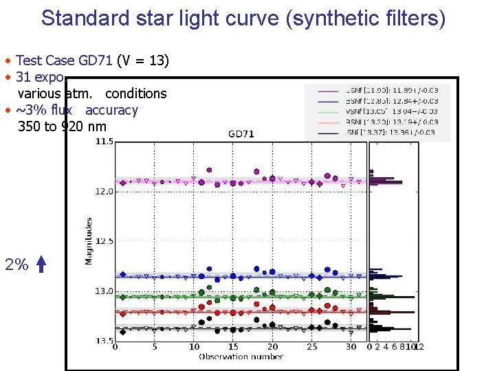
Standard star light curve (synthetic filters) • Test Case GD 71 (V = 13) • 31 expo. various atm. conditions • ~3% flux accuracy 350 to 920 nm 2%

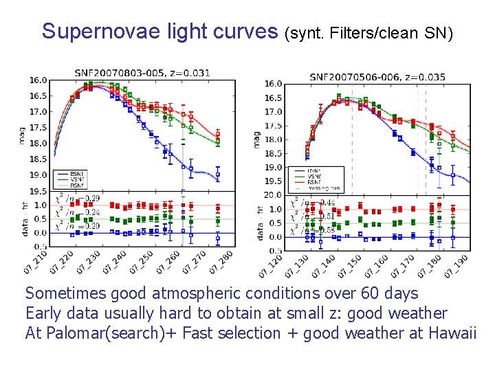
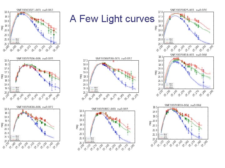
Supernovae light curves (synt. Filters/clean SN) Sometimes good atmospheric conditions over 60 days Early data usually hard to obtain at small z: good weather At Palomar(search)+ Fast selection + good weather at Hawaii

A Few Light curves

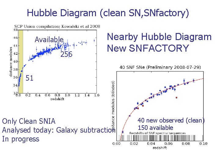
Hubble Diagram (clean SN, SNfactory) Available 256 Nearby Hubble Diagram New SNFACTORY 51 Only Clean SNIA Analysed today: Galaxy subtraction In progress 40 new observed (clean) 150 available

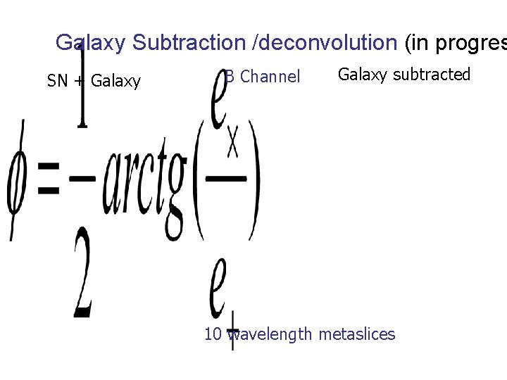
Galaxy Subtraction /deconvolution (in progres SN + Galaxy B Channel Galaxy subtracted 10 wavelength metaslices

Subtracted SN spectrum

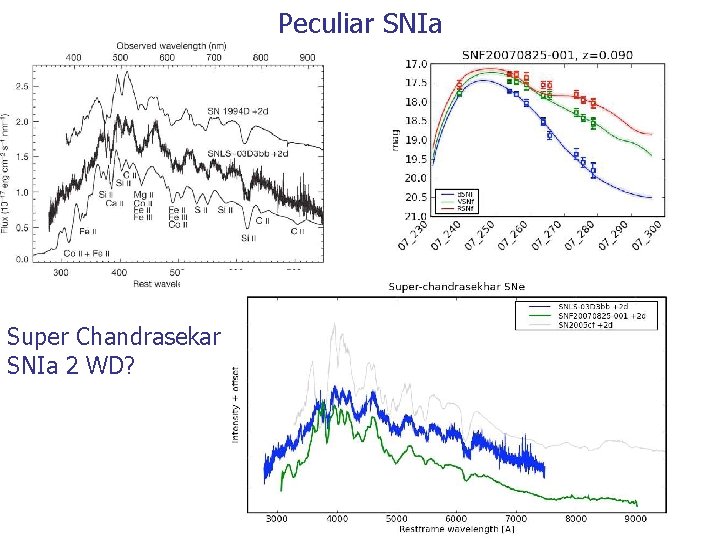
Peculiar SNIa Super Chandrasekar SNIa 2 WD?

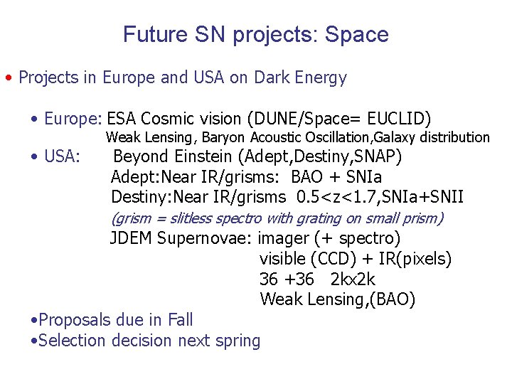
Future SN projects: Space • Projects in Europe and USA on Dark Energy • Europe: ESA Cosmic vision (DUNE/Space= EUCLID) Weak Lensing, Baryon Acoustic Oscillation, Galaxy distribution • USA: Beyond Einstein (Adept, Destiny, SNAP) Adept: Near IR/grisms: BAO + SNIa Destiny: Near IR/grisms 0. 5<z<1. 7, SNIa+SNII (grism = slitless spectro with grating on small prism) JDEM Supernovae: imager (+ spectro) visible (CCD) + IR(pixels) 36 +36 2 kx 2 k Weak Lensing, (BAO) • Proposals due in Fall • Selection decision next spring

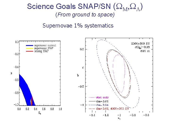
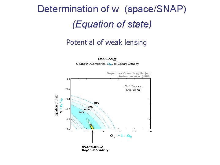
Science Goals SNAP/SN (WM, WL) (From ground to space) Supernovae 1% systematics

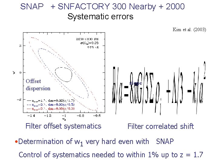
SNAP + SNFACTORY 300 Nearby + 2000 Systematic errors Kim et al. (2003) Offset dispersion slope Filter offset systematics Filter correlated shift • Determination of w 1 very hard even with SNAP Control of systematics needed to within 1% up to z = 1. 7

Control of systematic errors in SNAP • Challenging • Filters must be controlled to a few 10 -3 (despite ageing/cosmic rays + solar eruptions) • Good monitoring of pointing and PSF (Flux) • Detailed monitoring of detector behaviour (Temperature stability, non linearity, Persistence, response maps, interpixel Properties, intrapixelproperties, etc…) • Cross-check by other methods desirable

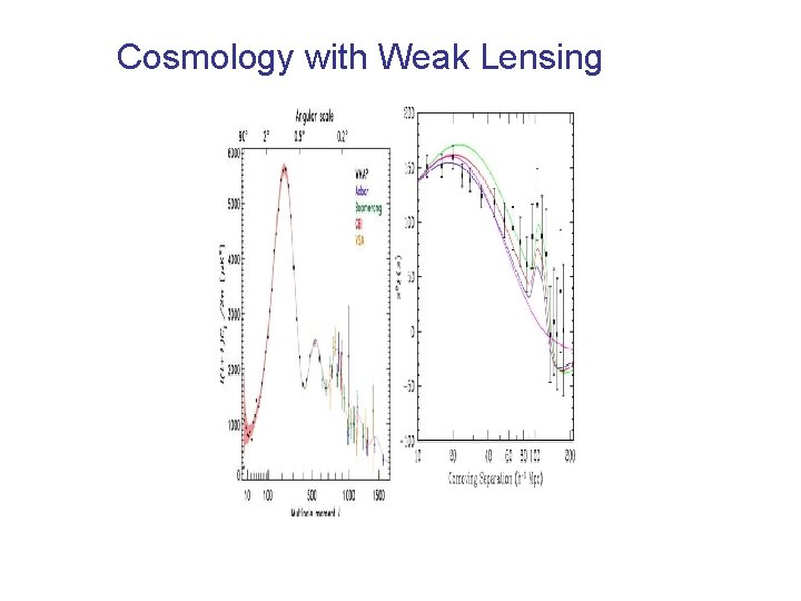
Cosmology with Weak Lensing

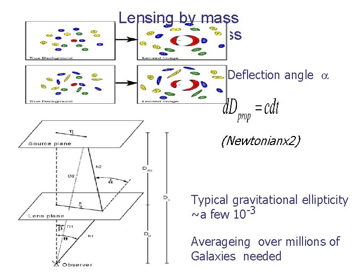
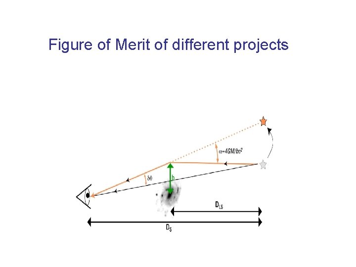
Lensing by mass Deflection angle a (Newtonianx 2) Typical gravitational ellipticity ~a few 10 -3 Averageing over millions of Galaxies needed

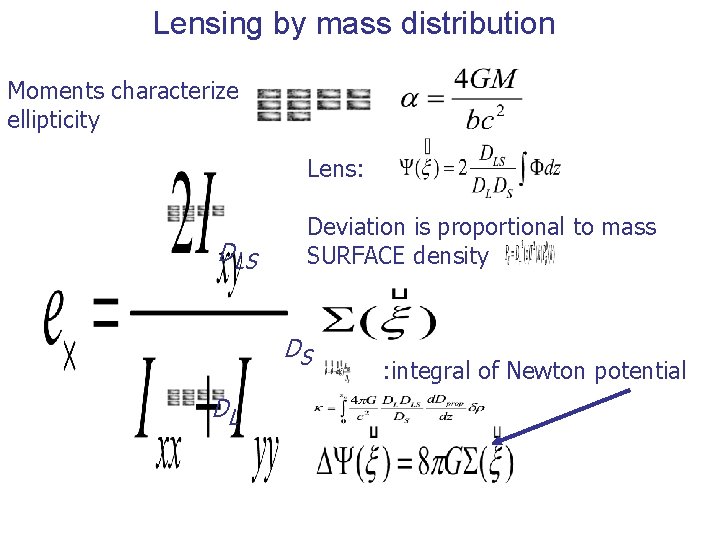
Lensing by mass distribution Moments characterize ellipticity Lens: DLS Deviation is proportional to mass SURFACE density DS : integral of Newton potential DL

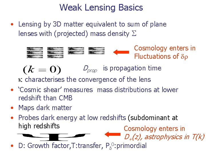
Weak Lensing Basics • Lensing by 3 D matter equivalent to sum of plane lenses with (projected) mass density S Cosmology enters in Fluctuations of dr Dprop is propagation time k characterises the convergence of the lens • ‘Cosmic shear’ measures mass distributions at lower redshift than CMB • Maps dark matter • Probes dark energy at low redshifts (subdominant at high redshifts Cosmology enters in D+(z), astrophysics in T(k) • D: Growth factor, T: transfer, Pd 0: primordial

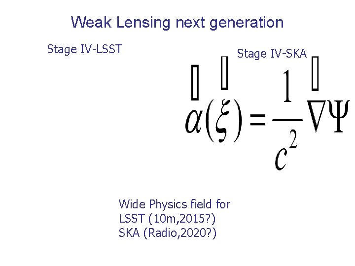
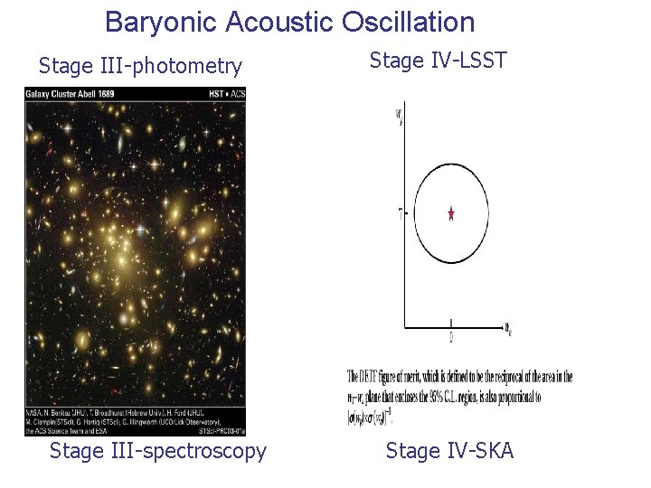
Weak Lensing next generation Stage IV-LSST Wide Physics field for LSST (10 m, 2015? ) SKA (Radio, 2020? ) Stage IV-SKA

Determination of w (space/SNAP) (Equation of state) Potential of weak lensing

Weak lensing systematics • Mainsystematic is linked to instrumental/atmospheric PSF • Telescope distorsions generate ‘fake’ distorsion correlations, must be corrected • Effect is much larger than gravitational lensing (a few 10 -3) • Need to control optical PSF to 10 -7 (including pointing) For w measurement • ‘at the edge’

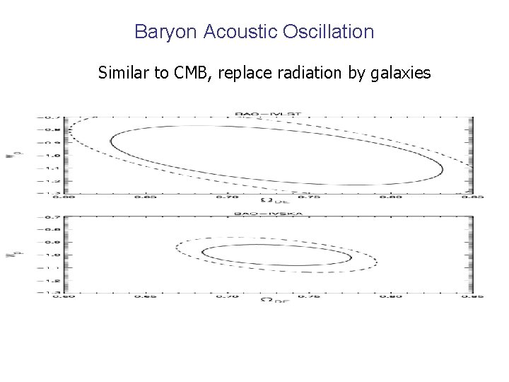
Baryon Acoustic Oscillation Similar to CMB, replace radiation by galaxies

Baryonic Acoustic Oscillation Stage III-photometry Stage III-spectroscopy Stage IV-LSST Stage IV-SKA

Conclusions • SNIa is now a ‘mature’ probe, although not fully understood. • Space experiments needed for progress on cosmology/SN • Even in space, constraining dark energy with SNIa will be difficult • Other techniques: BAO promising, lots of room for improvements, not very sensitive to L • Weak lensing: powerful, tough systematics/PSF • CMB: not really sensitive to L • Universe is a ‘relevant’ laboratory

Back Up

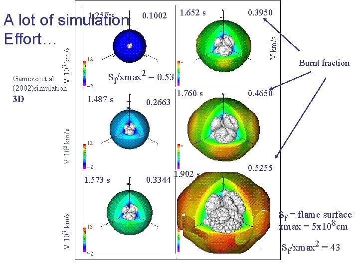
V 103 km/s A lot of simulation Effort… 12 -2 3 D 1. 487 s V 103 km/s 0. 3950 Burnt fraction Sf/xmax 2 = 0. 53 Gamezo et al. (2002)simulation 0. 2663 1. 760 s 0. 4650 12 -2 1. 573 s V 103 km/s 1. 652 s 0. 1002 V km/s 1. 257 s 12 -2 0. 3344 1. 902 s 0. 5255 Sf = flame surface xmax = 5 x 108 cm Sf/xmax 2 = 43

Figure of Merit of different projects