STELLAR MASSES AND THE HERTZSPRUNGRUSSELL DIAGRAM Mass is

STELLAR MASSES AND THE HERTZSPRUNGRUSSELL DIAGRAM Mass is the most important stellar property, but can only be found directly from binary star systems. We classify stars by their luminosities and temperatures.

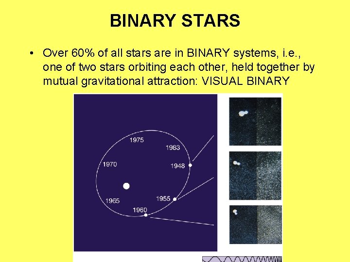
BINARY STARS • Over 60% of all stars are in BINARY systems, i. e. , one of two stars orbiting each other, held together by mutual gravitational attraction: VISUAL BINARY

CLASSIFICATION OF BINARIES • FALSE -- optical doubles -- these are close together in the sky, but well separated in distance and not bound by gravity. • TRUE are much more numerous! • Visual binaries -- relatively widely separated stars that can be seen by eye (a few) or telescope (lots); they appear to be close together, and ARE so. • Interferometric binaries -- only seen as two stars using speckle interferometry or actual interferometry: closer. • Composite spectrum binaries -- even through a telescope they appear to be just one star, but the spectrum shows two humps, implying two photospheres. • Astrometric binaries -- wiggly motion ACROSS the sky (determined similarly to parallax and proper motion) indicates gravitational tug of an unseen companion -- either another star or even a planet.

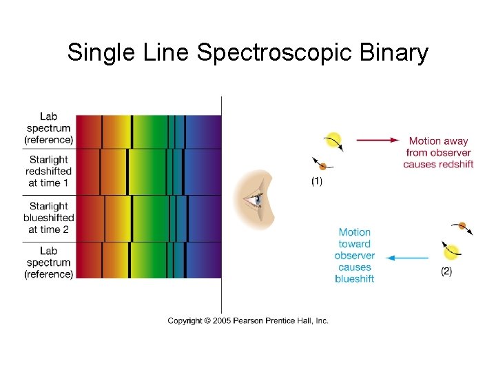
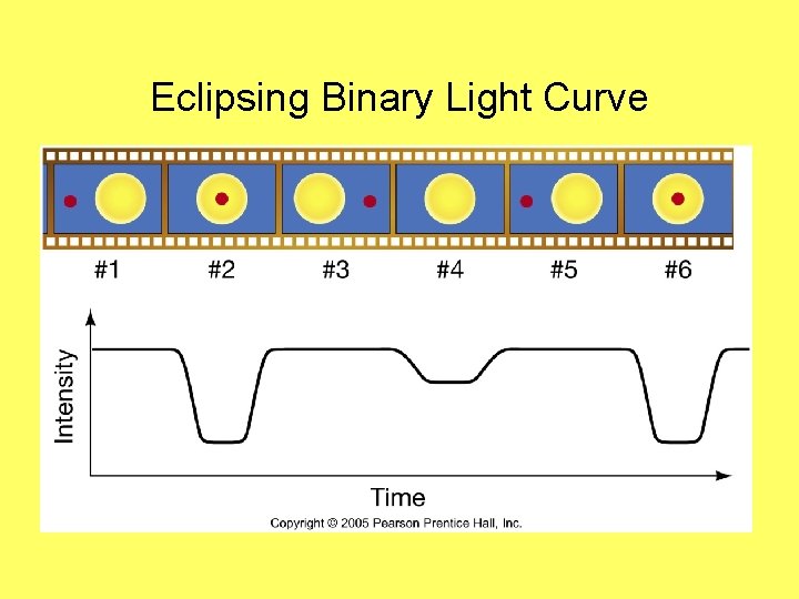
Most Important Binary Types • SPECTROSCOPIC binaries -- these are very useful close binaries and come in two classes: • Single-line spectroscopic -- the lines of only one star are seen, but they shift back and forth in wavelength, indicating orbital motion about a much fainter companion (usually a star, occasionally a planet); • Double-line spectroscopic -- orbital motion is detected in the spectra of BOTH stars; while one approaches, the other recedes. • ECLIPSING binaries -- close enough and with orbital plane near the line of sight, so stars alternately (at least partially) cover each other up; therefore the LIGHT CURVE undergoes dips.

Single Line Spectroscopic Binary

Eclipsing Binary Light Curve

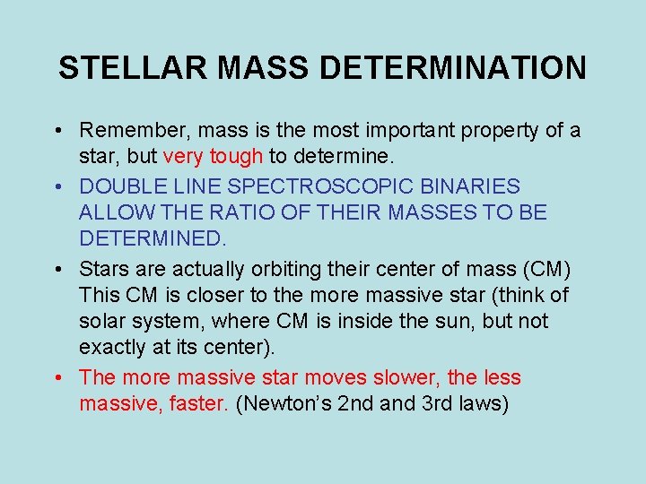
STELLAR MASS DETERMINATION • Remember, mass is the most important property of a star, but very tough to determine. • DOUBLE LINE SPECTROSCOPIC BINARIES ALLOW THE RATIO OF THEIR MASSES TO BE DETERMINED. • Stars are actually orbiting their center of mass (CM) This CM is closer to the more massive star (think of solar system, where CM is inside the sun, but not exactly at its center). • The more massive star moves slower, the less massive, faster. (Newton’s 2 nd and 3 rd laws)

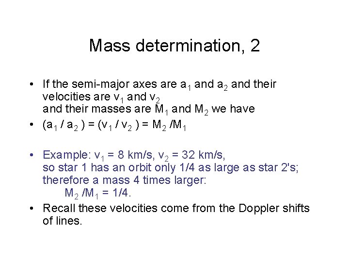
Mass determination, 2 • If the semi-major axes are a 1 and a 2 and their velocities are v 1 and v 2 and their masses are M 1 and M 2 we have • (a 1 / a 2 ) = (v 1 / v 2 ) = M 2 /M 1 • Example: v 1 = 8 km/s, v 2 = 32 km/s, so star 1 has an orbit only 1/4 as large as star 2's; therefore a mass 4 times larger: M 2 /M 1 = 1/4. • Recall these velocities come from the Doppler shifts of lines.

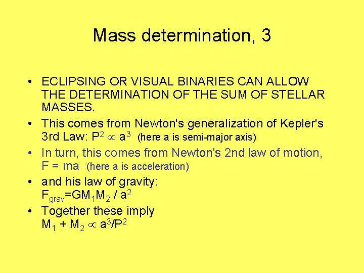
Mass determination, 3 • ECLIPSING OR VISUAL BINARIES CAN ALLOW THE DETERMINATION OF THE SUM OF STELLAR MASSES. • This comes from Newton's generalization of Kepler's 3 rd Law: P 2 a 3 (here a is semi-major axis) • In turn, this comes from Newton's 2 nd law of motion, F = ma (here a is acceleration) • and his law of gravity: Fgrav=GM 1 M 2 / a 2 • Together these imply M 1 + M 2 a 3/P 2

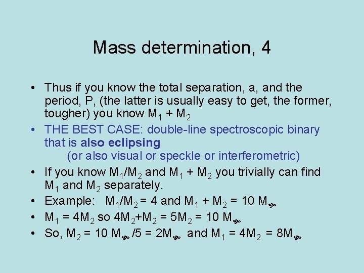
Mass determination, 4 • Thus if you know the total separation, a, and the period, P, (the latter is usually easy to get, the former, tougher) you know M 1 + M 2 • THE BEST CASE: double-line spectroscopic binary that is also eclipsing (or also visual or speckle or interferometric) • If you know M 1/M 2 and M 1 + M 2 you trivially can find M 1 and M 2 separately. • Example: M 1/M 2 = 4 and M 1 + M 2 = 10 M • M 1 = 4 M 2 so 4 M 2+M 2 = 5 M 2 = 10 M • So, M 2 = 10 M /5 = 2 M and M 1 = 4 M 2 = 8 M

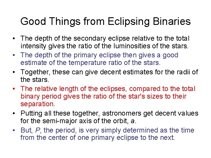
Good Things from Eclipsing Binaries • The depth of the secondary eclipse relative to the total intensity gives the ratio of the luminosities of the stars. • The depth of the primary eclipse then gives a good estimate of the temperature ratio of the stars. • Together, these can give decent estimates for the radii of the stars. • The relative length of the eclipses, compared to the total binary period gives the ratio of the star's sizes to their separation. • Putting all these together, astronomers get decent values for the semi-major axis of the orbit, a. • But, P, the period, is very simply determined as the time from the center of one primary eclipse to the next.

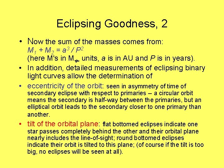
Eclipsing Goodness, 2 • Now the sum of the masses comes from: M 1 + M 2 = a 3 / P 2 (here M's in M units, a is in AU and P is in years). • In addition, detailed measurements of eclipsing binary light curves allow the determination of • eccentricity of the orbit: seen in asymmetry of time of secondary eclipse with respect to primaries -- a circular orbit means the secondary is half-way between the primaries, but an elliptical orbit leads to the secondary closer to one primary than another. • tilt of the orbital plane: flat bottomed eclipses indicate one star passes completely behind the other and their orbital plane nearly includes the line-of-sight; round bottomed eclipses indicate their orbit is tilted to this plane; (of course if the tilt is too big, no eclipses will be seen at all).

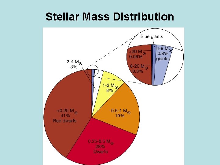
Stellar Mass Distribution

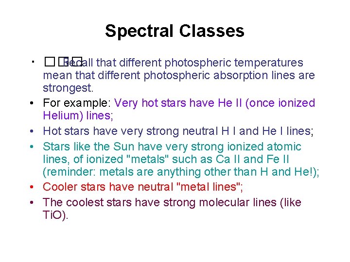
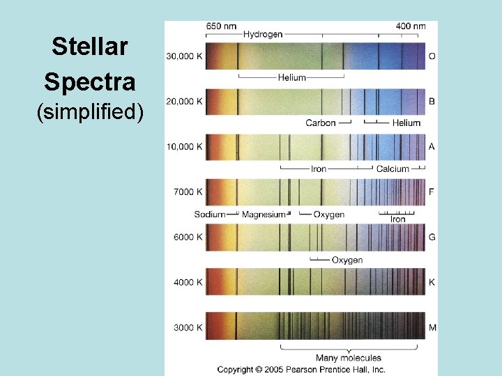
Spectral Classes • ��� Recall that different photospheric temperatures • • • mean that different photospheric absorption lines are strongest. For example: Very hot stars have He II (once ionized Helium) lines; Hot stars have very strong neutral H I and He I lines; Stars like the Sun have very strong ionized atomic lines, of ionized "metals" such as Ca II and Fe II (reminder: metals are anything other than H and He!); Cooler stars have neutral "metal lines"; The coolest stars have strong molecular lines (like Ti. O).

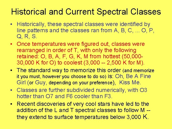
Historical and Current Spectral Classes • Historically, these spectral classes were identified by line patterns and the classes ran from A, B, C, . . . O, P, Q, R, S. • Once temperatures were figured out, classes were rearranged in order of T, with only the following retained: O, B, A, F, G, K, M from hottest (50, 00030, 000 K for O) to coolest (3, 000 -- 2, 500 K for M). • The standard way to memorize this order (and memorize it you must, however you choose to do so) is: Oh, Be A Fine Girl (or Guy, depending on your preference), Kiss Me. • Classes are further subdivided numerically, with O 3 hotter than O 7 and F 6 cooler than F 3. • Recent discoveries of very cool stars have led to the addition of the L and T spectral classes to follow M -they extend to surface temperatures below 3, 000 K.

Stellar Spectra (simplified)

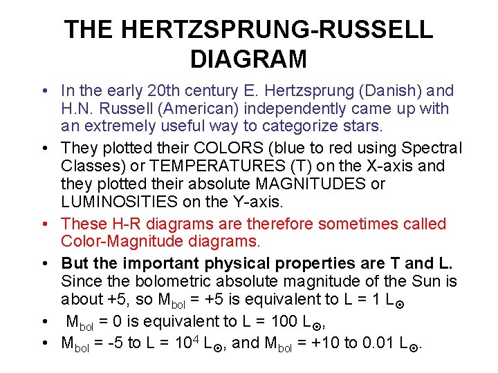
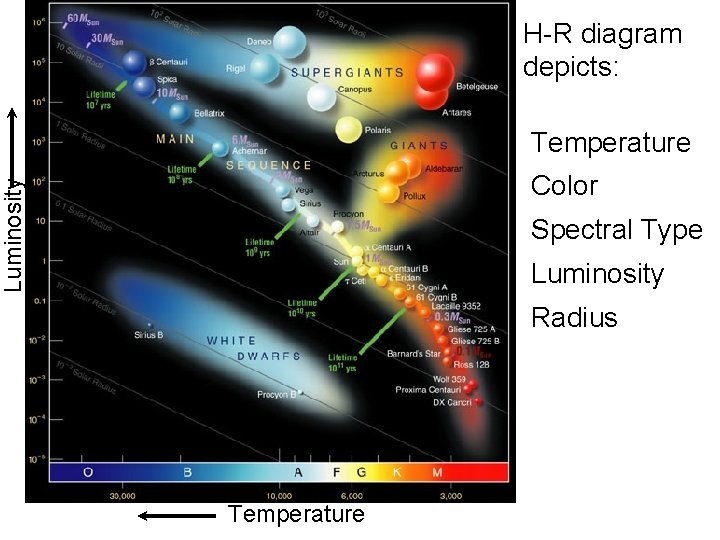
THE HERTZSPRUNG-RUSSELL DIAGRAM • In the early 20 th century E. Hertzsprung (Danish) and H. N. Russell (American) independently came up with an extremely useful way to categorize stars. • They plotted their COLORS (blue to red using Spectral Classes) or TEMPERATURES (T) on the X-axis and they plotted their absolute MAGNITUDES or LUMINOSITIES on the Y-axis. • These H-R diagrams are therefore sometimes called Color-Magnitude diagrams. • But the important physical properties are T and L. Since the bolometric absolute magnitude of the Sun is about +5, so Mbol = +5 is equivalent to L = 1 L • Mbol = 0 is equivalent to L = 100 L , • Mbol = -5 to L = 104 L , and Mbol = +10 to 0. 01 L.

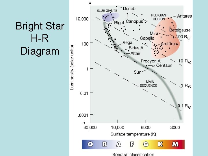
Bright Star H-R Diagram

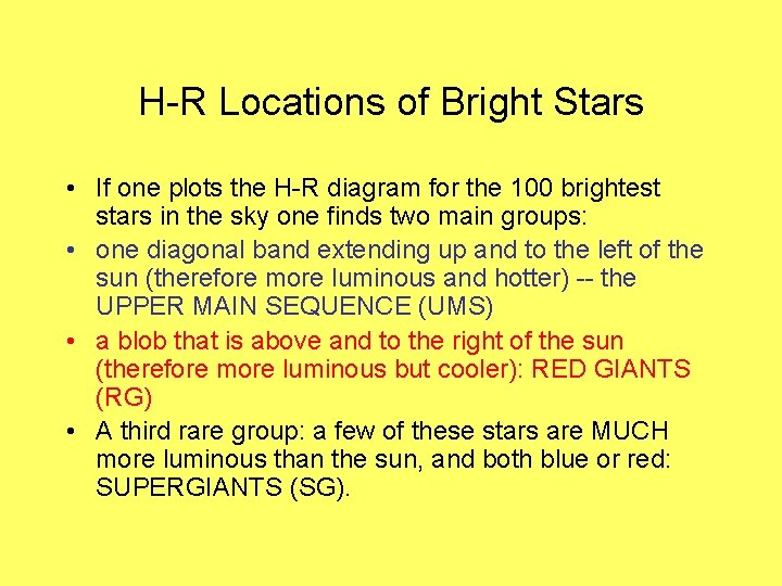
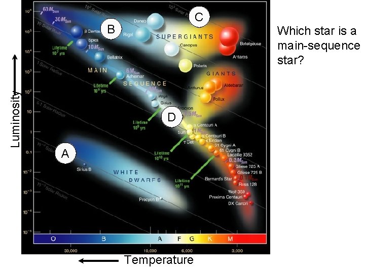
H-R Locations of Bright Stars • If one plots the H-R diagram for the 100 brightest stars in the sky one finds two main groups: • one diagonal band extending up and to the left of the sun (therefore more luminous and hotter) -- the UPPER MAIN SEQUENCE (UMS) • a blob that is above and to the right of the sun (therefore more luminous but cooler): RED GIANTS (RG) • A third rare group: a few of these stars are MUCH more luminous than the sun, and both blue or red: SUPERGIANTS (SG).

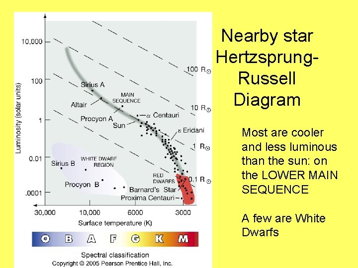
Nearby star Hertzsprung. Russell Diagram Most are cooler and less luminous than the sun: on the LOWER MAIN SEQUENCE A few are White Dwarfs

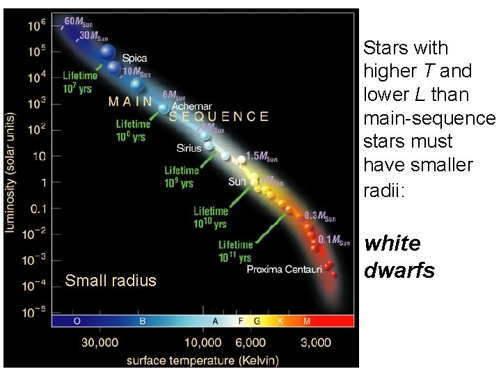
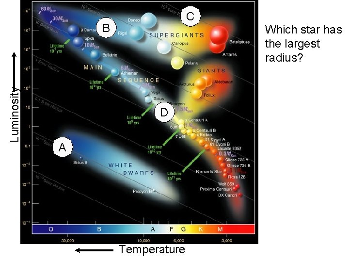
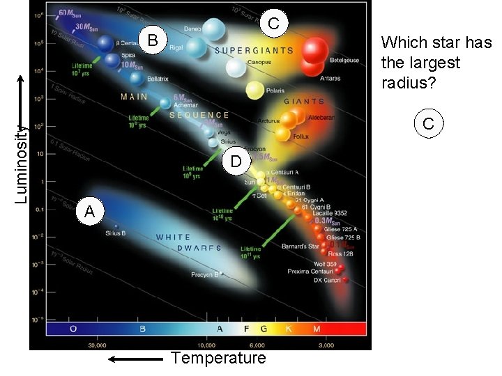
Representative Star H-R Diagram • But if one plots a MORE REPRESENTATIVE group of stars, say the 100 nearest to the sun, then a different pattern emerges on H-R diagrams. • The majority are in an extension of the UMS band, but to the right and below the sun (cooler and fainter) -- THE LOWER MAIN SEQUENCE (LMS) • another significant band is found to be below and to the left of the sun -- WHITE DWARFS (WD). • Lines of constant radius run diagonally from upper left to lower right in H-R diagrams, with the biggest stars in the UR corner and the smallest in the LL corner.

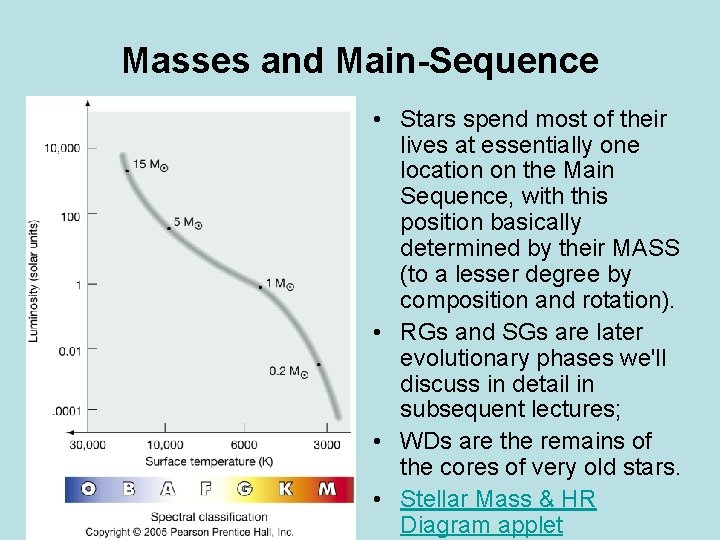
Masses and Main-Sequence • Stars spend most of their lives at essentially one location on the Main Sequence, with this position basically determined by their MASS (to a lesser degree by composition and rotation). • RGs and SGs are later evolutionary phases we'll discuss in detail in subsequent lectures; • WDs are the remains of the cores of very old stars. • Stellar Mass & HR Diagram applet

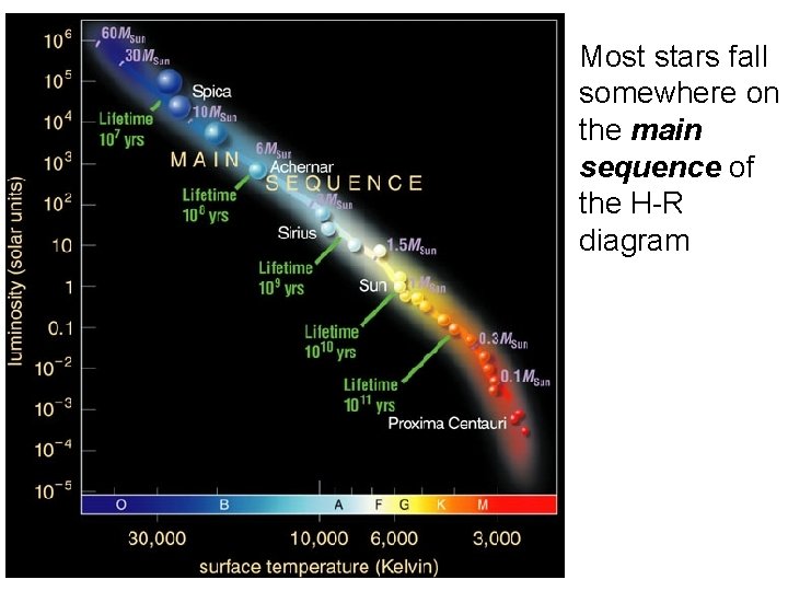
Most stars fall somewhere on the main sequence of the H-R diagram

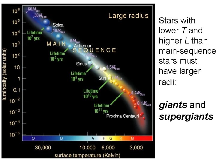
Large radius Stars with lower T and higher L than main-sequence stars must have larger radii: giants and supergiants

Stars with higher T and lower L than main-sequence stars must have smaller radii: Small radius white dwarfs

H-R diagram depicts: Temperature Luminosity Color Spectral Type Luminosity Radius Temperature

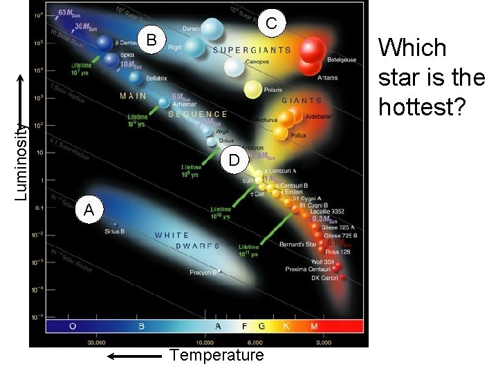
C Luminosity B Which star is the hottest? D A Temperature

C Luminosity B Which star is the hottest? D A A Temperature

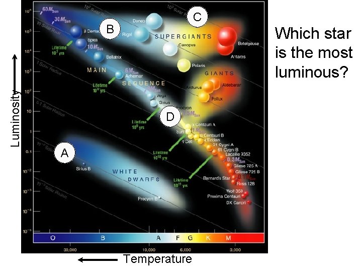
C Luminosity B Which star is the most luminous? D A Temperature

C Luminosity B Which star is the most luminous? C D A Temperature

C Luminosity B Which star is a main-sequence star? D A Temperature

C Luminosity B Which star is a main-sequence star? D D A Temperature

C Luminosity B Which star has the largest radius? D A Temperature

C Luminosity B Which star has the largest radius? C D A Temperature

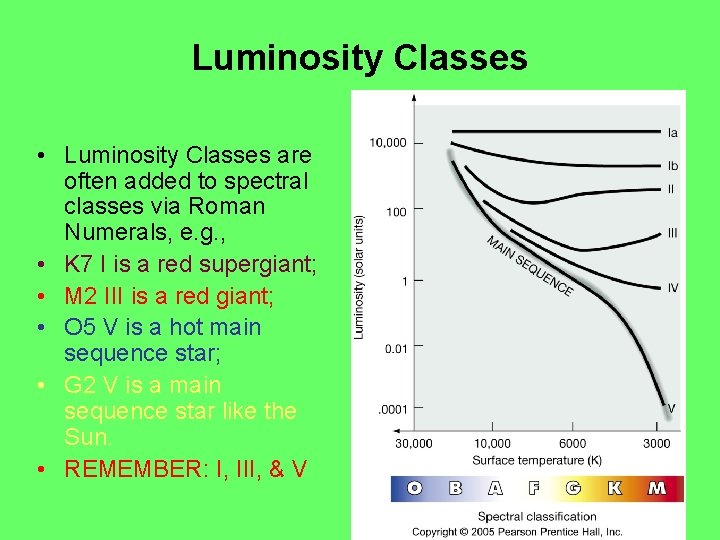
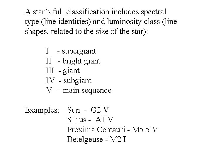
Luminosity Classes • Luminosity Classes are often added to spectral classes via Roman Numerals, e. g. , • K 7 I is a red supergiant; • M 2 III is a red giant; • O 5 V is a hot main sequence star; • G 2 V is a main sequence star like the Sun. • REMEMBER: I, III, & V

A star’s full classification includes spectral type (line identities) and luminosity class (line shapes, related to the size of the star): I - supergiant II - bright giant III - giant IV - subgiant V - main sequence Examples: Sun - G 2 V Sirius - A 1 V Proxima Centauri - M 5. 5 V Betelgeuse - M 2 I

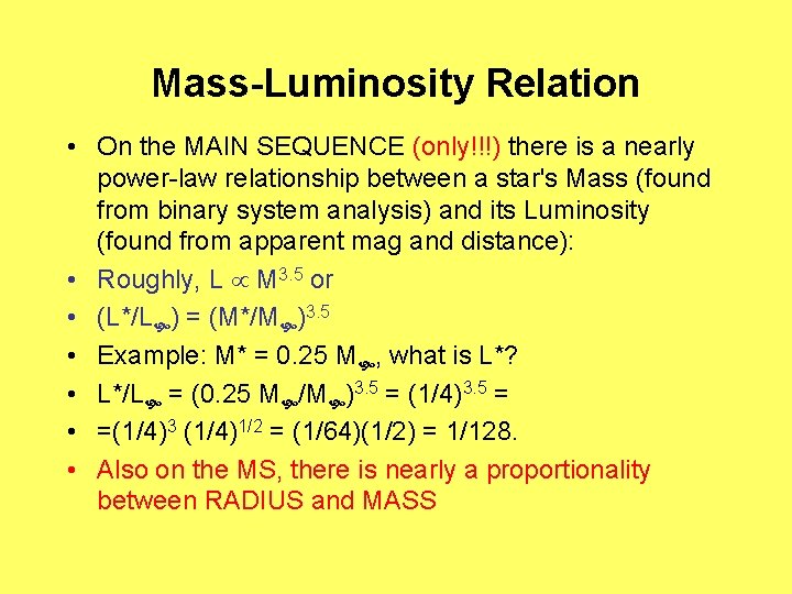
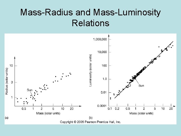
Mass-Luminosity Relation • On the MAIN SEQUENCE (only!!!) there is a nearly power-law relationship between a star's Mass (found from binary system analysis) and its Luminosity (found from apparent mag and distance): • Roughly, L M 3. 5 or • (L*/L ) = (M*/M )3. 5 • Example: M* = 0. 25 M , what is L*? • L*/L = (0. 25 M /M )3. 5 = (1/4)3. 5 = • =(1/4)3 (1/4)1/2 = (1/64)(1/2) = 1/128. • Also on the MS, there is nearly a proportionality between RADIUS and MASS

Mass-Radius and Mass-Luminosity Relations

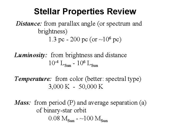
Stellar Properties Review Distance: from parallax angle (or spectrum and brightness) 1. 3 pc - 200 pc (or ~106 pc) Luminosity: from brightness and distance 10 -4 LSun - 106 LSun Temperature: from color (better: spectral type) 3, 000 K - 50, 000 K Mass: from period (P) and average separation (a) of binary-star orbit 0. 08 MSun - ~100 MSun