Statistical Design of Experiments SECTION VI RESPONSE SURFACE

Statistical Design of Experiments SECTION VI RESPONSE SURFACE METHODOLOGY Dr. Gary Blau, Sean Han Monday, Aug 13, 2007

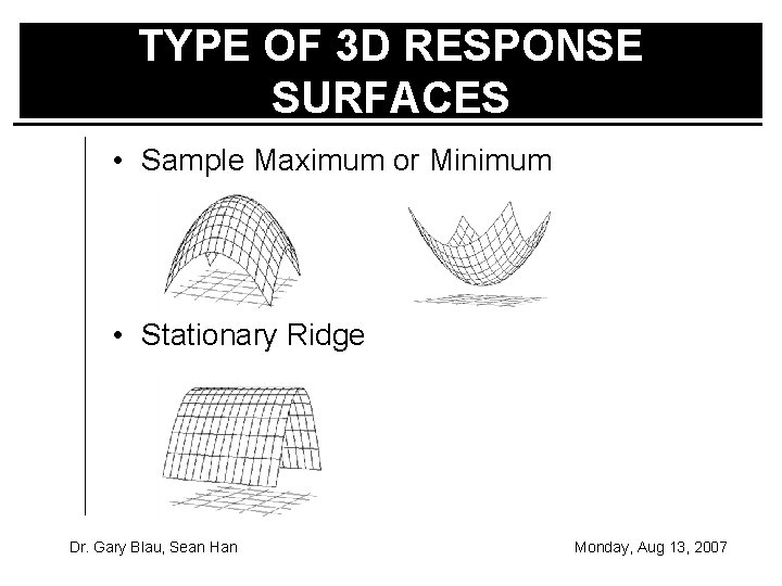
TYPE OF 3 D RESPONSE SURFACES • Sample Maximum or Minimum • Stationary Ridge Dr. Gary Blau, Sean Han Monday, Aug 13, 2007

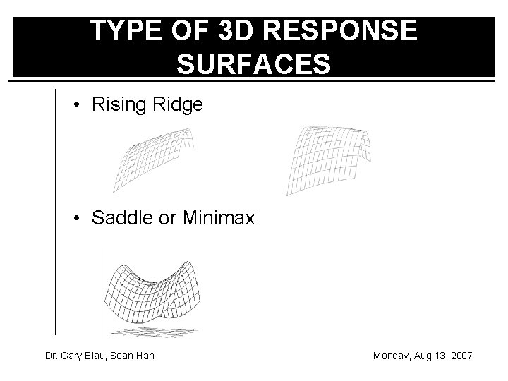
TYPE OF 3 D RESPONSE SURFACES • Rising Ridge • Saddle or Minimax Dr. Gary Blau, Sean Han Monday, Aug 13, 2007

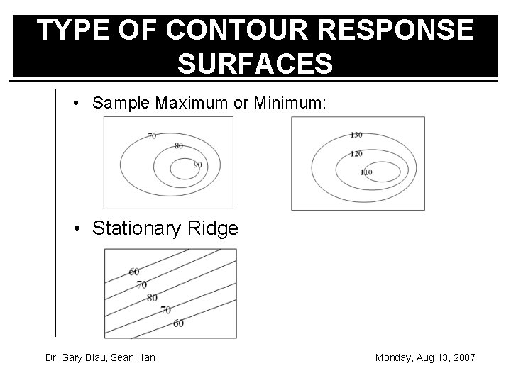
TYPE OF CONTOUR RESPONSE SURFACES • Sample Maximum or Minimum: • Stationary Ridge Dr. Gary Blau, Sean Han Monday, Aug 13, 2007

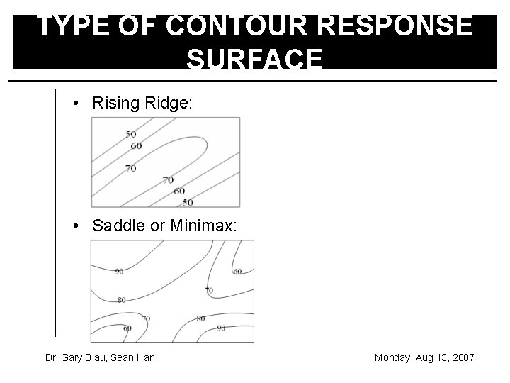
TYPE OF CONTOUR RESPONSE SURFACE • Rising Ridge: • Saddle or Minimax: Dr. Gary Blau, Sean Han Monday, Aug 13, 2007

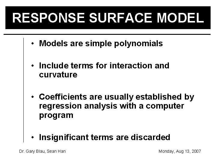
RESPONSE SURFACE MODEL • Models are simple polynomials • Include terms for interaction and curvature • Coefficients are usually established by regression analysis with a computer program • Insignificant terms are discarded Dr. Gary Blau, Sean Han Monday, Aug 13, 2007

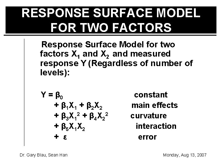
RESPONSE SURFACE MODEL FOR TWO FACTORS Response Surface Model for two factors X 1 and X 2 and measured response Y (Regardless of number of levels): Y = β 0 + β 1 X 1 + β 2 X 2 + β 3 X 12 + β 4 X 22 + β 5 X 1 X 2 + ε Dr. Gary Blau, Sean Han constant main effects curvature interaction error Monday, Aug 13, 2007

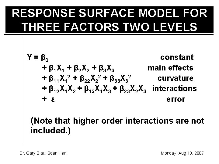
RESPONSE SURFACE MODEL FOR THREE FACTORS TWO LEVELS Y = β 0 constant + β 1 X 1 + β 2 X 2 + β 3 X 3 main effects + β 11 X 12 + β 22 X 22 + β 33 X 32 curvature + β 12 X 1 X 2 + β 13 X 1 X 3 + β 23 X 2 X 3 interactions + ε error (Note that higher order interactions are not included. ) Dr. Gary Blau, Sean Han Monday, Aug 13, 2007

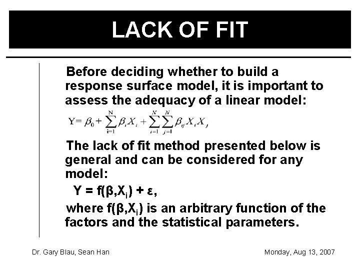
LACK OF FIT Before deciding whether to build a response surface model, it is important to assess the adequacy of a linear model: The lack of fit method presented below is general and can be considered for any model: Y = f(β, Xi) + ε, where f(β, Xi) is an arbitrary function of the factors and the statistical parameters. Dr. Gary Blau, Sean Han Monday, Aug 13, 2007

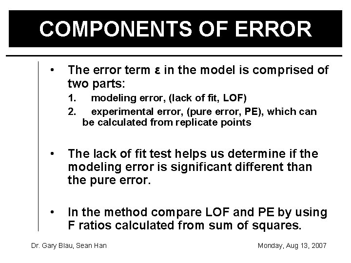
COMPONENTS OF ERROR • The error term ε in the model is comprised of two parts: 1. 2. modeling error, (lack of fit, LOF) experimental error, (pure error, PE), which can be calculated from replicate points • The lack of fit test helps us determine if the modeling error is significant different than the pure error. • In the method compare LOF and PE by using F ratios calculated from sum of squares. Dr. Gary Blau, Sean Han Monday, Aug 13, 2007

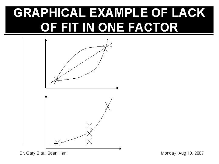
GRAPHICAL EXAMPLE OF LACK OF FIT IN ONE FACTOR Dr. Gary Blau, Sean Han Monday, Aug 13, 2007

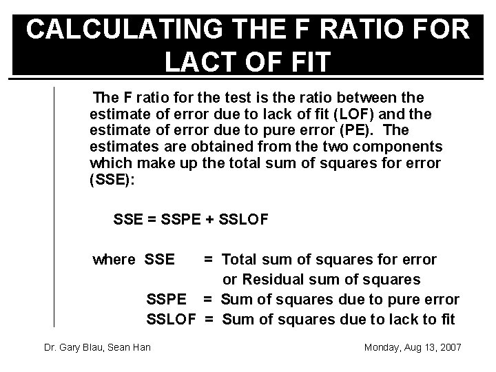
CALCULATING THE F RATIO FOR LACT OF FIT The F ratio for the test is the ratio between the estimate of error due to lack of fit (LOF) and the estimate of error due to pure error (PE). The estimates are obtained from the two components which make up the total sum of squares for error (SSE): SSE = SSPE + SSLOF where SSE = Total sum of squares for error or Residual sum of squares SSPE = Sum of squares due to pure error SSLOF = Sum of squares due to lack to fit Dr. Gary Blau, Sean Han Monday, Aug 13, 2007

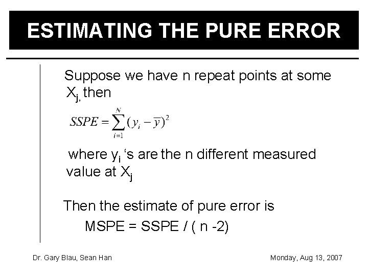
ESTIMATING THE PURE ERROR Suppose we have n repeat points at some Xj, then where yi ‘s are the n different measured value at Xj Then the estimate of pure error is MSPE = SSPE / ( n -2) Dr. Gary Blau, Sean Han Monday, Aug 13, 2007

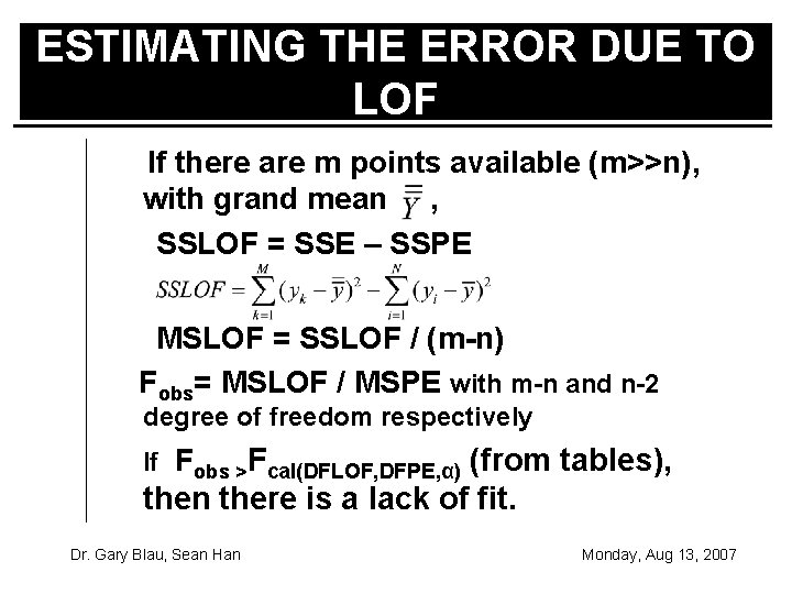
ESTIMATING THE ERROR DUE TO LOF If there are m points available (m>>n), with grand mean , SSLOF = SSE – SSPE MSLOF = SSLOF / (m-n) Fobs= MSLOF / MSPE with m-n and n-2 degree of freedom respectively If Fobs >Fcal(DFLOF, DFPE, α) (from tables), then there is a lack of fit. Dr. Gary Blau, Sean Han Monday, Aug 13, 2007

LACK OF FIT TEST FOR SEVERAL POINTS REPEATED When several points are repeated, the general approach is to determine the SSPE for each set of replicates and then “pool” these sum of squares by forming an overall SSPE weighted by the degree of freedom for each set. Then the estimate of PE is obtained by dividing the SSPE by the appropriate number of degree of freedom and continuing as above. Dr. Gary Blau, Sean Han Monday, Aug 13, 2007

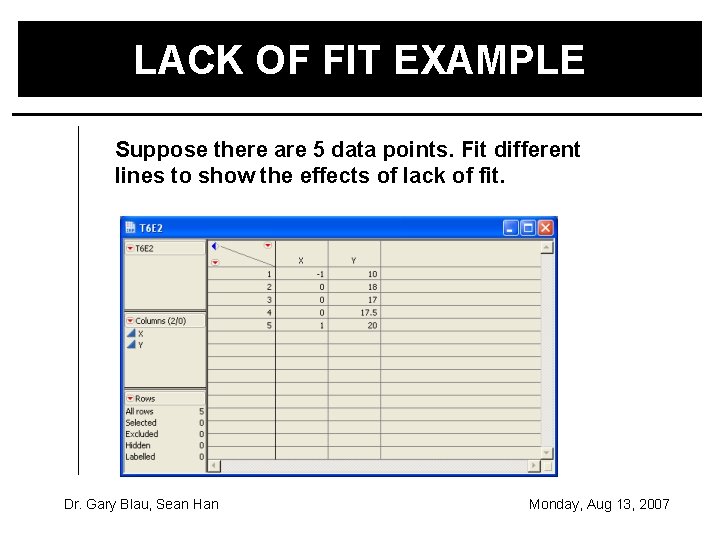
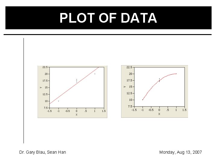
LACK OF FIT EXAMPLE Suppose there are 5 data points. Fit different lines to show the effects of lack of fit. Dr. Gary Blau, Sean Han Monday, Aug 13, 2007

PLOT OF DATA Dr. Gary Blau, Sean Han Monday, Aug 13, 2007

TYPES OF RSM DESIGN • Three Level Factorial Experiments • Central Composite Designs (CCD) • Box Behnken Designs Dr. Gary Blau, Sean Han Monday, Aug 13, 2007

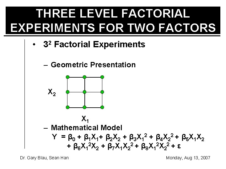
THREE LEVEL FACTORIAL EXPERIMENTS FOR TWO FACTORS • 32 Factorial Experiments – Geometric Presentation X 2 X 1 – Mathematical Model Y = β 0 + β 1 X 1+ β 2 X 2 + β 3 X 12 + β 4 X 22 + β 5 X 1 X 2 + β 6 X 12 X 2 + β 7 X 1 X 22 + β 8 X 12 X 22 + ε Dr. Gary Blau, Sean Han Monday, Aug 13, 2007

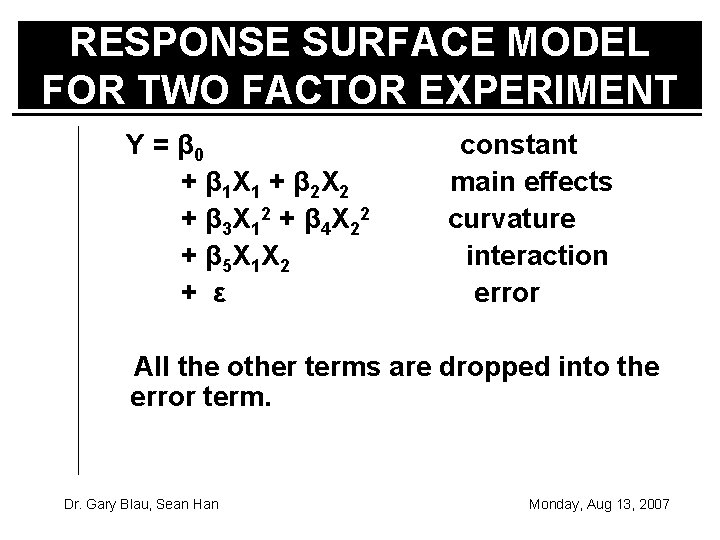
RESPONSE SURFACE MODEL FOR TWO FACTOR EXPERIMENT Y = β 0 + β 1 X 1 + β 2 X 2 + β 3 X 12 + β 4 X 22 + β 5 X 1 X 2 + ε constant main effects curvature interaction error All the other terms are dropped into the error term. Dr. Gary Blau, Sean Han Monday, Aug 13, 2007

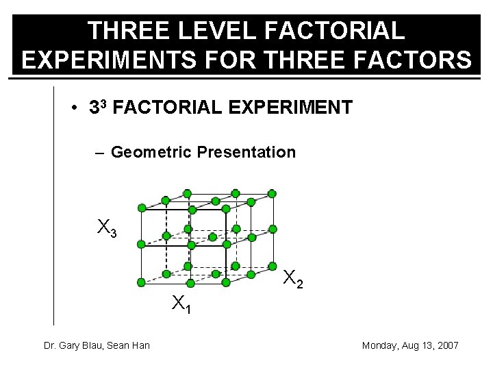
THREE LEVEL FACTORIAL EXPERIMENTS FOR THREE FACTORS • 33 FACTORIAL EXPERIMENT – Geometric Presentation X 3 X 2 X 1 Dr. Gary Blau, Sean Han Monday, Aug 13, 2007

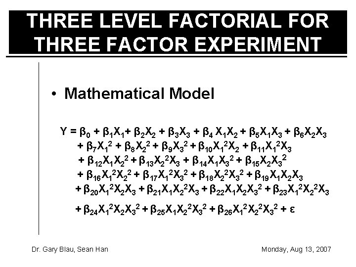
THREE LEVEL FACTORIAL FOR THREE FACTOR EXPERIMENT • Mathematical Model Y = β 0 + β 1 X 1+ β 2 X 2 + β 3 X 3 + β 4 X 1 X 2 + β 5 X 1 X 3 + β 6 X 2 X 3 + β 7 X 12 + β 8 X 22 + β 9 X 32 + β 10 X 12 X 2 + β 11 X 12 X 3 + β 12 X 1 X 22 + β 13 X 22 X 3 + β 14 X 1 X 32 + β 15 X 2 X 32 + β 16 X 12 X 22 + β 17 X 12 X 32 + β 18 X 22 X 32 + β 19 X 1 X 2 X 3 + β 20 X 12 X 2 X 3 + β 21 X 1 X 22 X 3 + β 22 X 1 X 2 X 32 + β 23 X 12 X 22 X 3 + β 24 X 12 X 2 X 32 + β 25 X 1 X 22 X 32 + β 26 X 12 X 22 X 32 + ε Dr. Gary Blau, Sean Han Monday, Aug 13, 2007

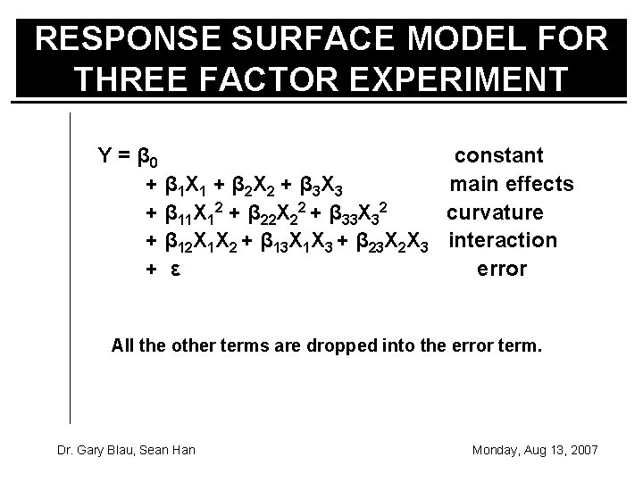
RESPONSE SURFACE MODEL FOR THREE FACTOR EXPERIMENT Y = β 0 constant + β 1 X 1 + β 2 X 2 + β 3 X 3 main effects + β 11 X 12 + β 22 X 22 + β 33 X 32 curvature + β 12 X 1 X 2 + β 13 X 1 X 3 + β 23 X 2 X 3 interaction + ε error All the other terms are dropped into the error term. Dr. Gary Blau, Sean Han Monday, Aug 13, 2007

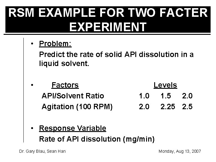
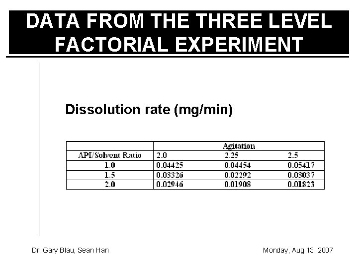
RSM EXAMPLE FOR TWO FACTER EXPERIMENT • Problem: Predict the rate of solid API dissolution in a liquid solvent. • Factors API/Solvent Ratio Agitation (100 RPM) Levels 1. 0 1. 5 2. 0 2. 25 2. 5 • Response Variable Rate of API dissolution (mg/min) Dr. Gary Blau, Sean Han Monday, Aug 13, 2007

DATA FROM THE THREE LEVEL FACTORIAL EXPERIMENT Dissolution rate (mg/min) Dr. Gary Blau, Sean Han Monday, Aug 13, 2007

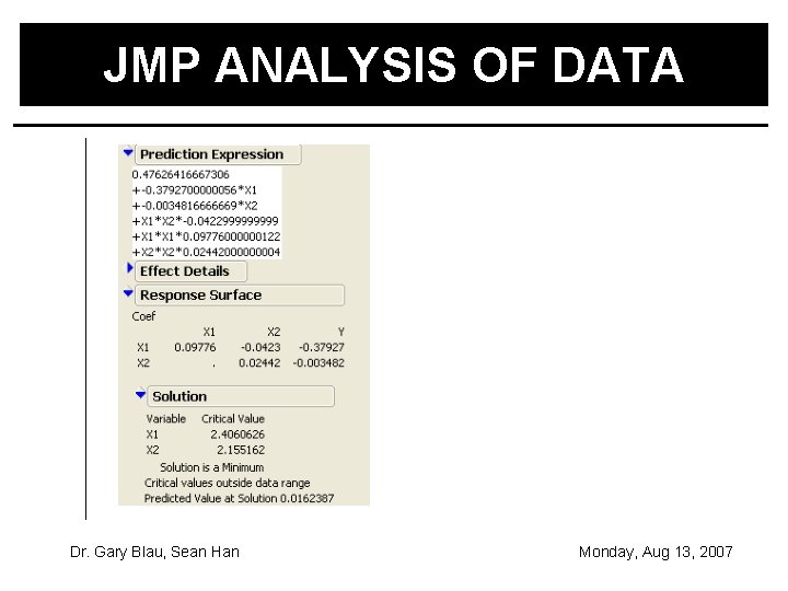
JMP ANALYSIS OF DATA Dr. Gary Blau, Sean Han Monday, Aug 13, 2007

NUMBER OF RUNS FOR A 3 k FACTORIAL EXPERIMENT • The number inside [brackets] is the number of runs needed for a third replicate of the full 3 k factorial experiment Dr. Gary Blau, Sean Han Monday, Aug 13, 2007

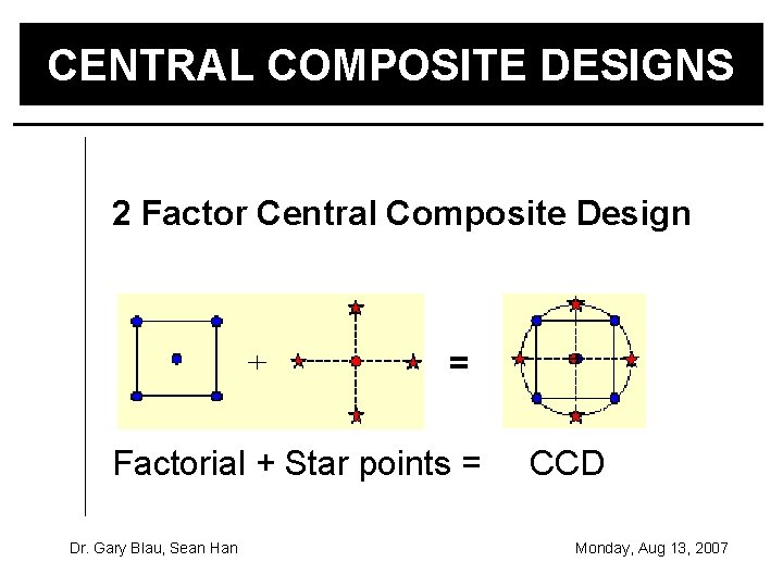
CENTRAL COMPOSITE DESIGNS 2 Factor Central Composite Design = Factorial + Star points = Dr. Gary Blau, Sean Han CCD Monday, Aug 13, 2007

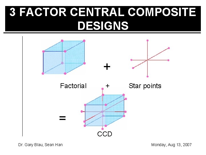
3 FACTOR CENTRAL COMPOSITE DESIGNS + Factorial + Star points = CCD Dr. Gary Blau, Sean Han Monday, Aug 13, 2007

CENTRAL COMPOSITE DESIGN • In a central composite design, each factor has 5 levels 1. 2. 3. 4. 5. extreme high (star point) high center low extreme low (star point) • The “hidden” factorial or fractional factorial experiment should be run first and analyzed • Depending on the results of a LOF test, the star points should be run next Dr. Gary Blau, Sean Han Monday, Aug 13, 2007

COMPARISON OF CCD WITH 3 k FACTORIAL EXPERIMENTS • Are as efficient as 3 k factorial experiments - minimum number of trials for estimating main effects and quadratic terms • Require less runs than 3 k factorial experiments • Allow sequential experimentation, which provides flexibility in running the experiment Dr. Gary Blau, Sean Han Monday, Aug 13, 2007

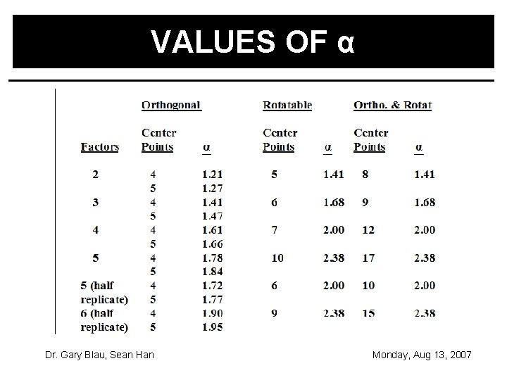
ORTHOGONAL CCD’S Orthogonal CCD’s can be constructed by taking α 1 = α 2 = …=αn and suitably choosing α. (Using JMP) Here α is the distance from the star points to the center point. (All star points lie a specific equal distance from the center of the circumscribing sphere. ) Orthogonal CCD’s assure no correlation among the effects being estimated. The value of α depends on whether or not the design is orthogonally blocked. That is, the question is whether or not the design is divided into blocks such that the block effects do not affect the estimates of the coefficients in the 2 nd order model. Dr. Gary Blau, Sean Han Monday, Aug 13, 2007

ROTATABLE CCD’S • Rotatable CCD’s are such that all points lie an equal distance from the center. (Hicks, 1964) (Star points lie on the sphere which circumscribes the factorial design. ) This type of CCD provides equal error prediction R units from the center, independent of direction. • In most cases, rotatable designs have a small correlation between the curvature terms. This correlation can be lessened by adding more center points. With enough center points, the design can be both orthogonal and rotatable. Dr. Gary Blau, Sean Han Monday, Aug 13, 2007

VALUES OF α Dr. Gary Blau, Sean Han Monday, Aug 13, 2007

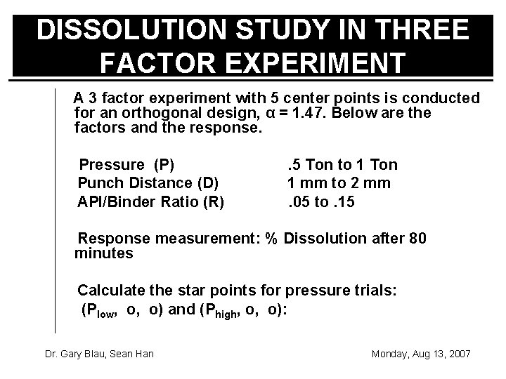
DISSOLUTION STUDY IN THREE FACTOR EXPERIMENT A 3 factor experiment with 5 center points is conducted for an orthogonal design, α = 1. 47. Below are the factors and the response. Pressure (P) Punch Distance (D) API/Binder Ratio (R) . 5 Ton to 1 Ton 1 mm to 2 mm. 05 to. 15 Response measurement: % Dissolution after 80 minutes Calculate the star points for pressure trials: (Plow, o, o) and (Phigh, o, o): Dr. Gary Blau, Sean Han Monday, Aug 13, 2007

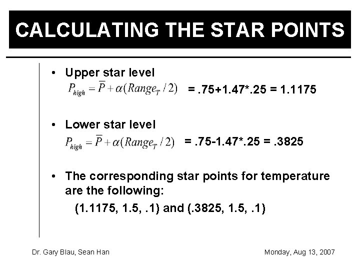
CALCULATING THE STAR POINTS • Upper star level =. 75+1. 47*. 25 = 1. 1175 • Lower star level =. 75 -1. 47*. 25 =. 3825 • The corresponding star points for temperature are the following: (1. 1175, 1. 5, . 1) and (. 3825, 1. 5, . 1) Dr. Gary Blau, Sean Han Monday, Aug 13, 2007

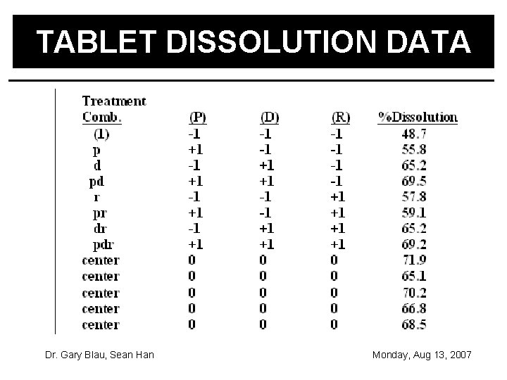
TABLET DISSOLUTION DATA Dr. Gary Blau, Sean Han Monday, Aug 13, 2007

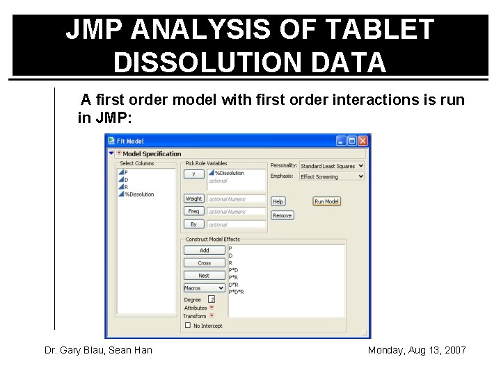
JMP ANALYSIS OF TABLET DISSOLUTION DATA A first order model with first order interactions is run in JMP: Dr. Gary Blau, Sean Han Monday, Aug 13, 2007

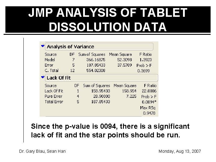
JMP ANALYSIS OF TABLET DISSOLUTION DATA Since the p-value is 0094, there is a significant lack of fit and the star points should be run. Dr. Gary Blau, Sean Han Monday, Aug 13, 2007

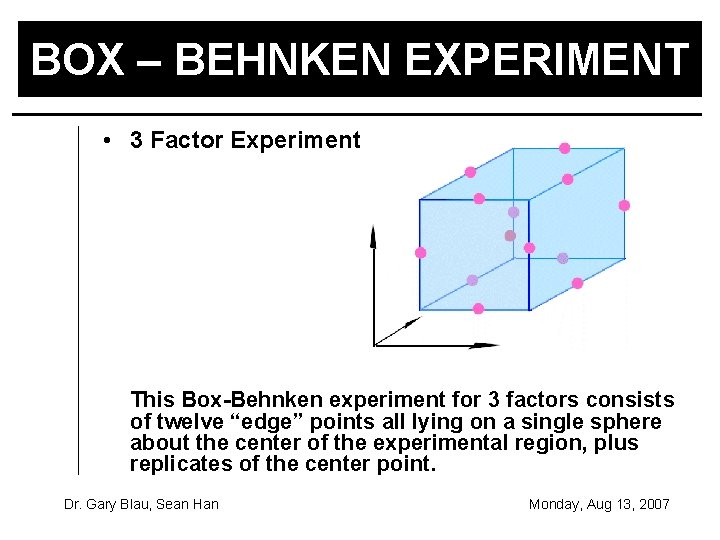
BOX – BEHNKEN EXPERIMENT • 3 Factor Experiment This Box-Behnken experiment for 3 factors consists of twelve “edge” points all lying on a single sphere about the center of the experimental region, plus replicates of the center point. Dr. Gary Blau, Sean Han Monday, Aug 13, 2007

BOX-BEHNKEN EXPERIMENT • • Is actually a portion of a 3 k factorial Three levels of each factor are used Center points should always be included It is possible to estimate main effects and second order terms • The experiments cannot be run sequentially as with CCD’s • Box-Behnken experiments are particularly useful if some boundary areas of the design region are infeasible, such as the extremes of the experiment region. Dr. Gary Blau, Sean Han Monday, Aug 13, 2007

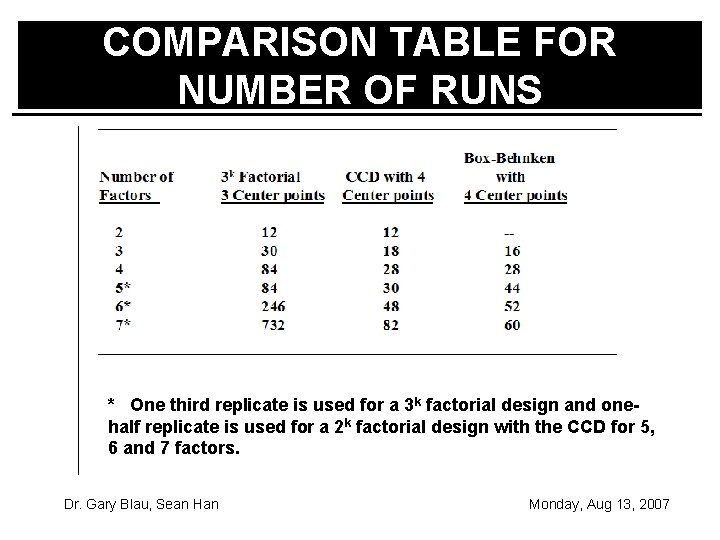
COMPARISON TABLE FOR NUMBER OF RUNS * One third replicate is used for a 3 k factorial design and onehalf replicate is used for a 2 k factorial design with the CCD for 5, 6 and 7 factors. Dr. Gary Blau, Sean Han Monday, Aug 13, 2007

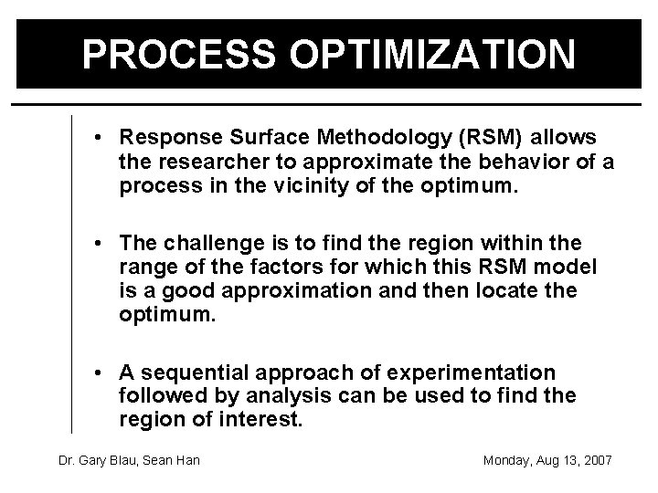
PROCESS OPTIMIZATION • Response Surface Methodology (RSM) allows the researcher to approximate the behavior of a process in the vicinity of the optimum. • The challenge is to find the region within the range of the factors for which this RSM model is a good approximation and then locate the optimum. • A sequential approach of experimentation followed by analysis can be used to find the region of interest. Dr. Gary Blau, Sean Han Monday, Aug 13, 2007

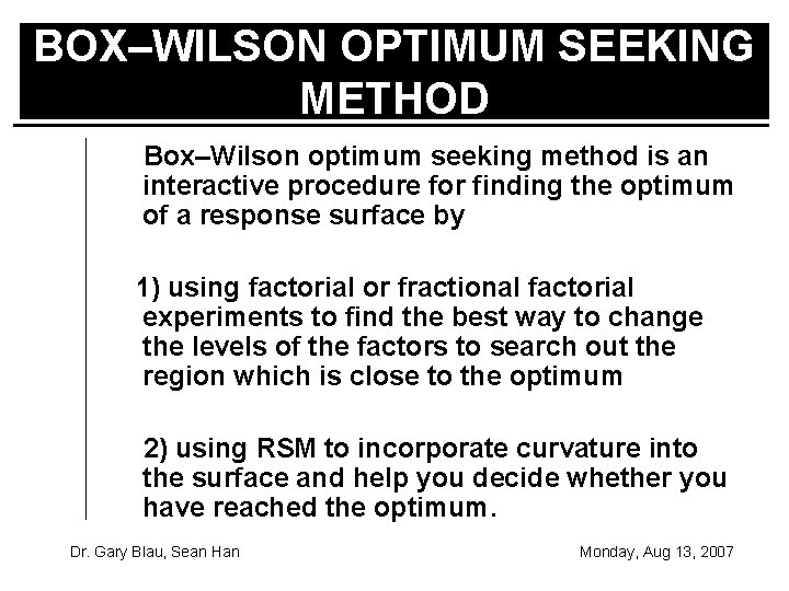
BOX–WILSON OPTIMUM SEEKING METHOD Box–Wilson optimum seeking method is an interactive procedure for finding the optimum of a response surface by 1) using factorial or fractional factorial experiments to find the best way to change the levels of the factors to search out the region which is close to the optimum 2) using RSM to incorporate curvature into the surface and help you decide whether you have reached the optimum. Dr. Gary Blau, Sean Han Monday, Aug 13, 2007

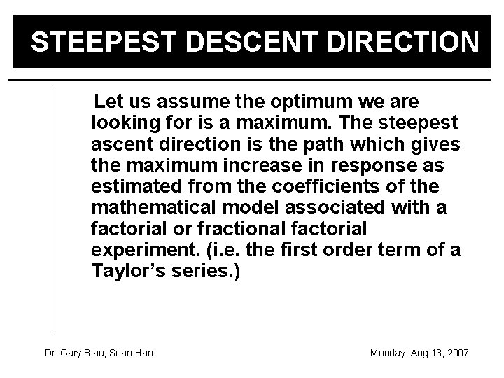
STEEPEST DESCENT DIRECTION Let us assume the optimum we are looking for is a maximum. The steepest ascent direction is the path which gives the maximum increase in response as estimated from the coefficients of the mathematical model associated with a factorial or fractional factorial experiment. (i. e. the first order term of a Taylor’s series. ) Dr. Gary Blau, Sean Han Monday, Aug 13, 2007

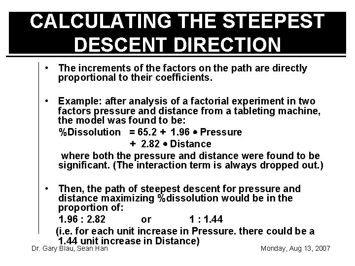
CALCULATING THE STEEPEST DESCENT DIRECTION • The increments of the factors on the path are directly proportional to their coefficients. • Example: after analysis of a factorial experiment in two factors pressure and distance from a tableting machine, the model was found to be: %Dissolution = 65. 2 + 1. 96 Pressure + 2. 82 Distance where both the pressure and distance were found to be significant. (The interaction term is always dropped out. ) • Then, the path of steepest descent for pressure and distance maximizing %dissolution would be in the proportion of: 1. 96 : 2. 82 or 1 : 1. 44 (i. e. for each unit increase in Pressure. there could be a 1. 44 unit increase in Distance) Dr. Gary Blau, Sean Han Monday, Aug 13, 2007

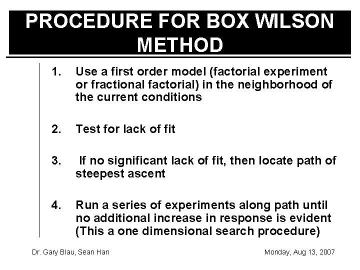
PROCEDURE FOR BOX WILSON METHOD 1. Use a first order model (factorial experiment or fractional factorial) in the neighborhood of the current conditions 2. Test for lack of fit 3. If no significant lack of fit, then locate path of steepest ascent 4. Run a series of experiments along path until no additional increase in response is evident (This a one dimensional search procedure) Dr. Gary Blau, Sean Han Monday, Aug 13, 2007

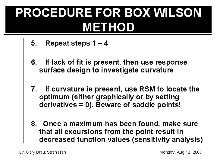
PROCEDURE FOR BOX WILSON METHOD 5. Repeat steps 1 – 4 6. If lack of fit is present, then use response surface design to investigate curvature 7. If curvature is present, use RSM to locate the optimum (either graphically or by setting derivatives = 0). Beware of saddle points! 8. Once a maximum has been found, make sure that all excursions from the point result in decreased function values (sensitivity analysis) Dr. Gary Blau, Sean Han Monday, Aug 13, 2007

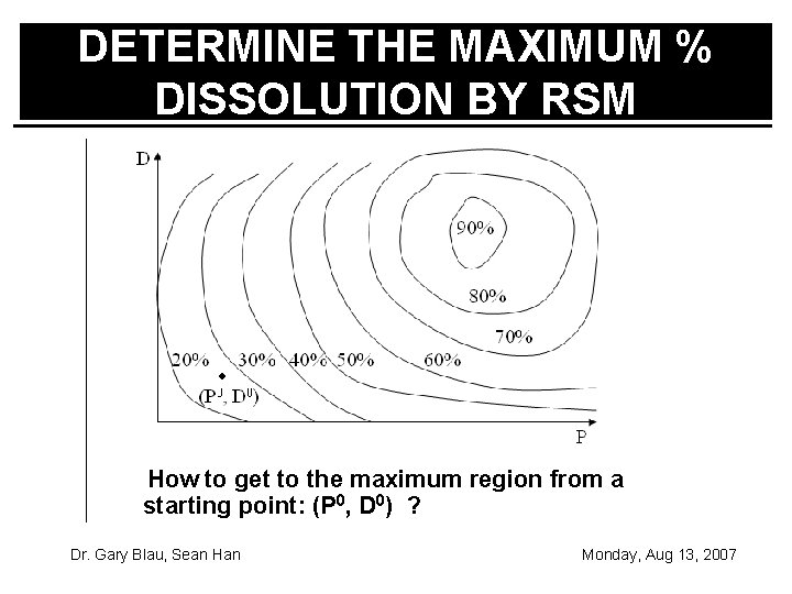
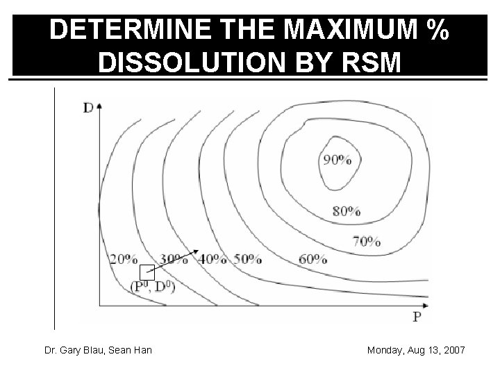
DETERMINE THE MAXIMUM % DISSOLUTION BY RSM How to get to the maximum region from a starting point: (P 0, D 0) ? Dr. Gary Blau, Sean Han Monday, Aug 13, 2007

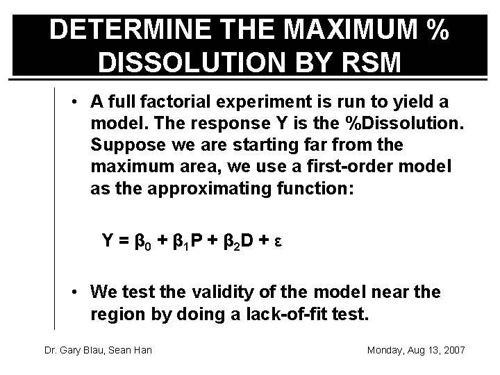
DETERMINE THE MAXIMUM % DISSOLUTION BY RSM • A full factorial experiment is run to yield a model. The response Y is the %Dissolution. Suppose we are starting far from the maximum area, we use a first-order model as the approximating function: Y = β 0 + β 1 P + β 2 D + ε • We test the validity of the model near the region by doing a lack-of-fit test. Dr. Gary Blau, Sean Han Monday, Aug 13, 2007

DETERMINE THE MAXIMUM % DISSOLUTION BY RSM Dr. Gary Blau, Sean Han Monday, Aug 13, 2007

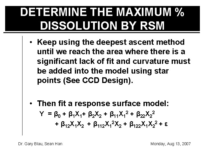
DETERMINE THE MAXIMUM % DISSOLUTION BY RSM • Keep using the deepest ascent method until we reach the area where there is a significant lack of fit and curvature must be added into the model using star points (See CCD Design). • Then fit a response surface model: Y = β 0 + β 1 X 1+ β 2 X 2 + β 11 X 12 + β 22 X 22 + β 12 X 1 X 2 + β 112 X 2 + β 122 X 1 X 22 + ε Dr. Gary Blau, Sean Han Monday, Aug 13, 2007

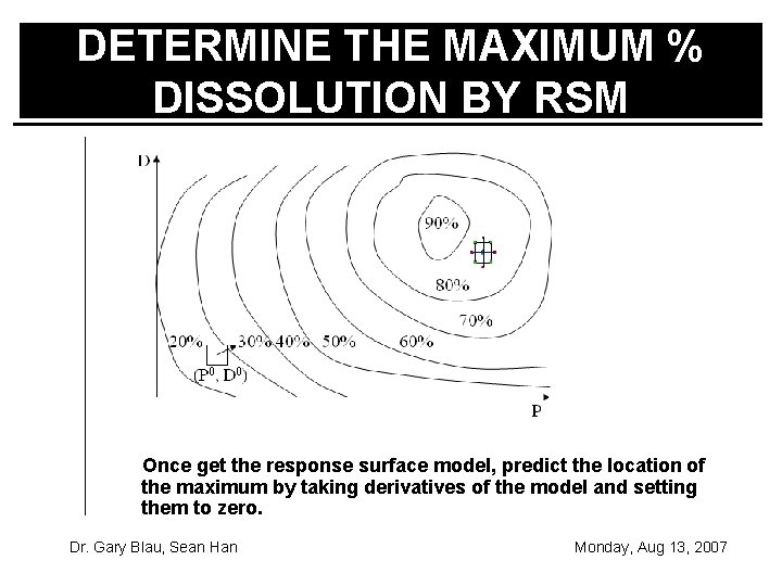
DETERMINE THE MAXIMUM % DISSOLUTION BY RSM Once get the response surface model, predict the location of the maximum by taking derivatives of the model and setting them to zero. Dr. Gary Blau, Sean Han Monday, Aug 13, 2007