Soft computing Lecture 7 MultiLayer perceptrons Why hidden

Soft computing Lecture 7 Multi-Layer perceptrons

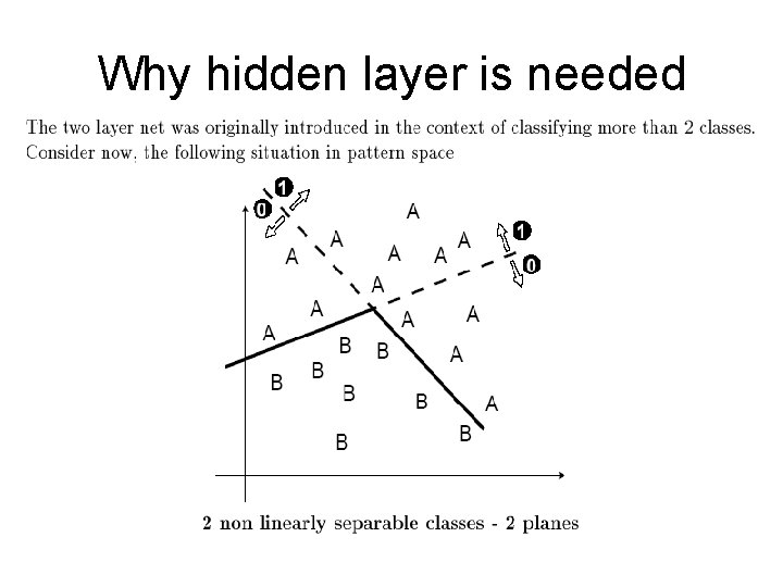
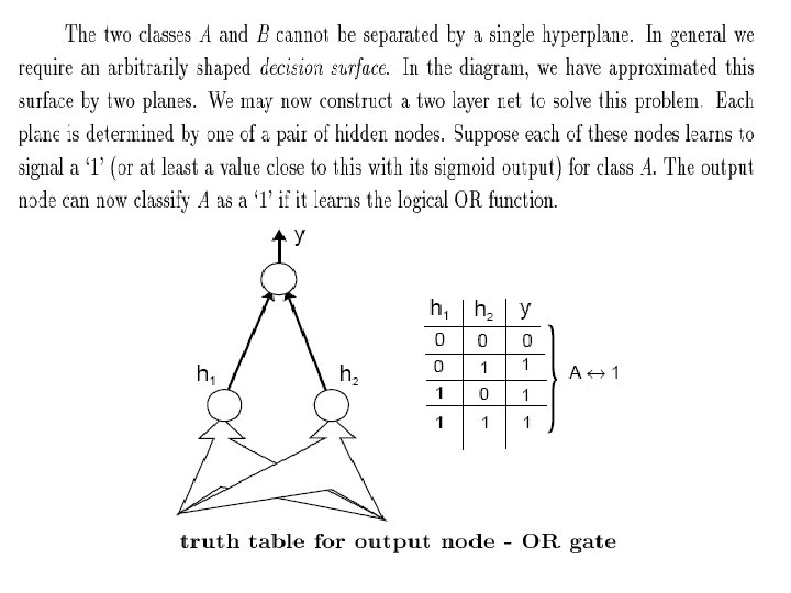
Why hidden layer is needed

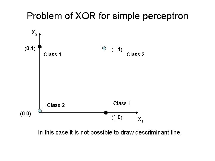
Problem of XOR for simple perceptron X 2 (0, 1) Class 1 Class 2 (0, 0) (1, 1) Class 2 Class 1 (1, 0) X 1 In this case it is not possible to draw descriminant line

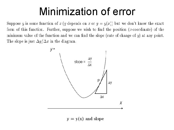
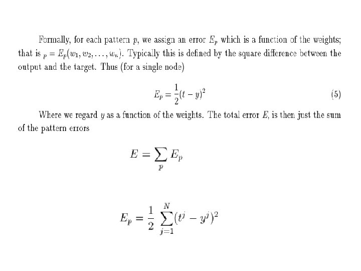
Minimization of error

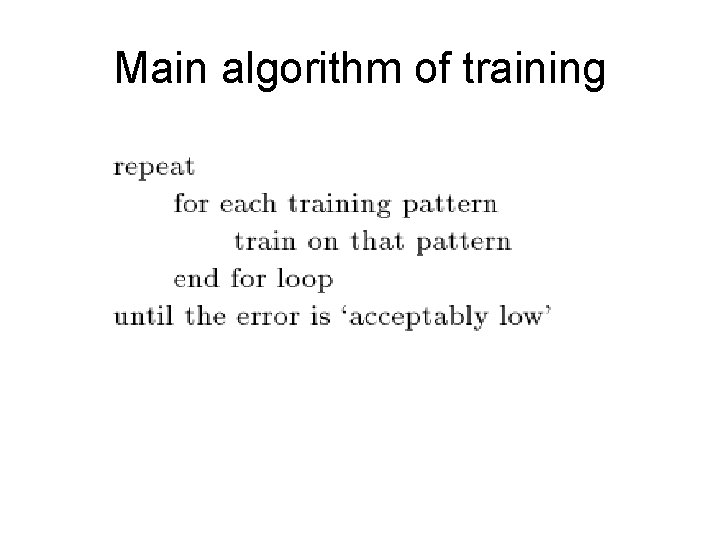
Main algorithm of training

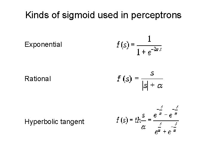
Kinds of sigmoid used in perceptrons Exponential Rational Hyperbolic tangent

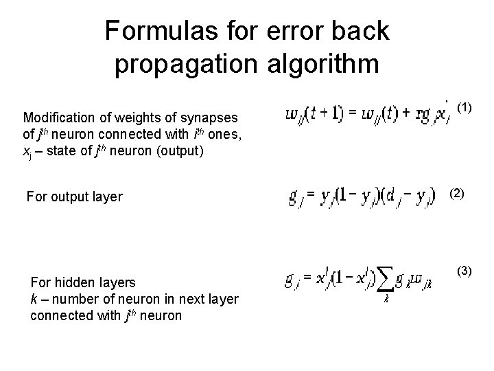
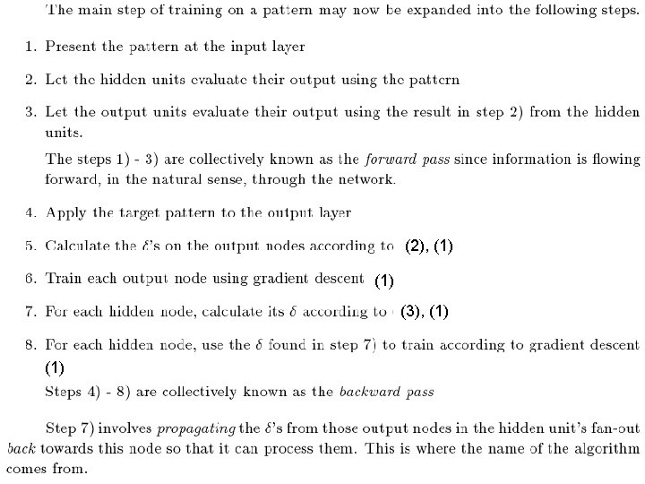
Formulas for error back propagation algorithm Modification of weights of synapses of jth neuron connected with ones, xj – state of jth neuron (output) For output layer For hidden layers k – number of neuron in next layer connected with jth neuron (1) (2) (3)

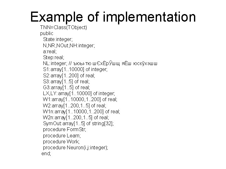
Example of implementation TNN=Class(TObject) public State: integer; N, NR, NOut, NH: integer; a: real; Step: real; NL: integer; // ъюы-тю шЄхЁрЎшщ яЁш юсєўхэшш S 1: array[1. . 10000] of integer; S 2: array[1. . 200] of real; S 3: array[1. . 5] of real; G 3: array[1. . 5] of real; LX, LY: array[1. . 10000] of integer; W 1: array[1. . 10000, 1. . 200] of real; W 2: array[1. . 200, 1. . 5] of real; W 1 n: array[1. . 10000, 1. . 200] of real; W 2 n: array[1. . 200, 1. . 5] of real; Sym. Out: array[1. . 5] of string[32]; procedure Form. Str; procedure Learn; procedure Work; procedure Neuron(i, j: integer); end;

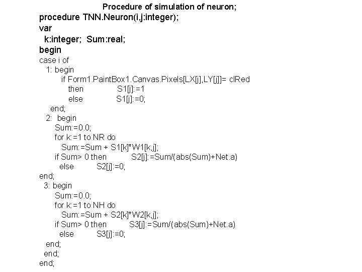
Procedure of simulation of neuron; procedure TNN. Neuron(i, j: integer); var k: integer; Sum: real; begin case i of 1: begin if Form 1. Paint. Box 1. Canvas. Pixels[LX[j], LY[j]]= cl. Red then S 1[j]: =1 else S 1[j]: =0; end; 2: begin Sum: =0. 0; for k: =1 to NR do Sum: =Sum + S 1[k]*W 1[k, j]; if Sum> 0 then S 2[j]: =Sum/(abs(Sum)+Net. a) else S 2[j]: =0; end; 3: begin Sum: =0. 0; for k: =1 to NH do Sum: =Sum + S 2[k]*W 2[k, j]; if Sum> 0 then S 3[j]: =Sum/(abs(Sum)+Net. a) else S 3[j]: =0; end;

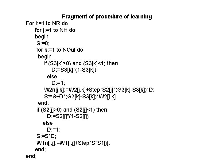
Fragment of procedure of learning For i: =1 to NR do for j: =1 to NH do begin S: =0; for k: =1 to NOut do begin if (S 3[k]>0) and (S 3[k]<1) then D: =S 3[k]*(1 -S 3[k]) else D: =1; W 2 n[j, k]: =W 2[j, k]+Step*S 2[j]*(G 3[k]-S 3[k])*D; S: =S+D*(G 3[k]-S 3[k])*W 2[j, k] end; if (S 2[j]>0) and (S 2[j]<1) then D: =S 2[j]*(1 -S 2[j]) else D: =1; S: =S*D; W 1 n[i, j]: =W 1[i, j]+Step*S*S 1[i]; end;

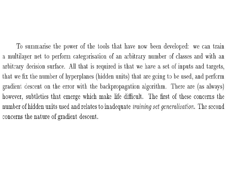
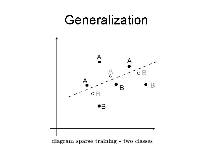
Generalization

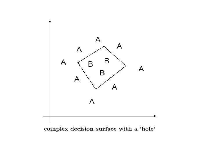
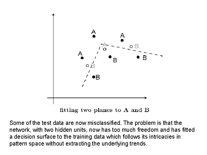
Some of the test data are now misclassified. The problem is that the network, with two hidden units, now has too much freedom and has fitted a decision surface to the training data which follows its intricacies in pattern space without extracting the underlying trends.

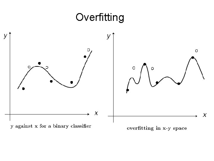
Overfitting

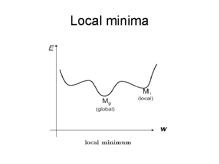
Local minima

Two tasks solved by MLP • Classification (recognition) – Usually binary outputs • Regression (approximation) – Analog outputs

Theorem of Kolmogorov “Any continuous function from input to output can be implemented in a three-layer net, given sufficient number of hidden units n. H, proper nonlinearities, and weights. ”

Advantages and disadvantages of MLP with back propagation • Advantages: – Guarantee of possibility of solving of tasks • Disadvantages: – Low speed of learning – Possibility of overfitting – Impossible to relearning – Selection of structure needed for solving of concrete task is unknown

Increase of speed of learning • Preliminary processing of features before getting to inputs of percepton • Dynamical step of learning (in begin one is large, than one is decreasing) • Using of second derivative in formulas for modification of weights • Using hardware implementation

Fight against of overfitting • Don’t select too small error for learning or too large number of iteration

Choice of structure • Using of constructive learning algorithms – Deleting of nodes (neurons) and links corresponding to one – Appending new neurons if it is needed • Using of genetic algorithms for selection of suboptimal structure

Impossible to relearning • Using of constructive learning algorithms – Deleting of nodes (neurons) and links corresponding to one – Appending new neurons if it is needed