Multilayer Perceptrons 1 ARTIFICIAL INTELLIGENCE TECHNIQUES Overview Recap

Multilayer Perceptrons 1 ARTIFICIAL INTELLIGENCE TECHNIQUES

Overview Recap of neural network theory The multi-layered perceptron Back-propagation Introduction to training Uses

Recap

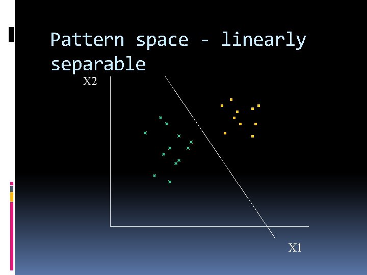
Linear separability When a neuron learns it is positioning a line so that all points on or above the line give an output of 1 and all points below the line give an output of 0 When there are more than 2 inputs, the pattern space is multi-dimensional, and is divided by a multi-dimensional surface (or hyperplane) rather than a line

Pattern space - linearly separable X 2 X 1

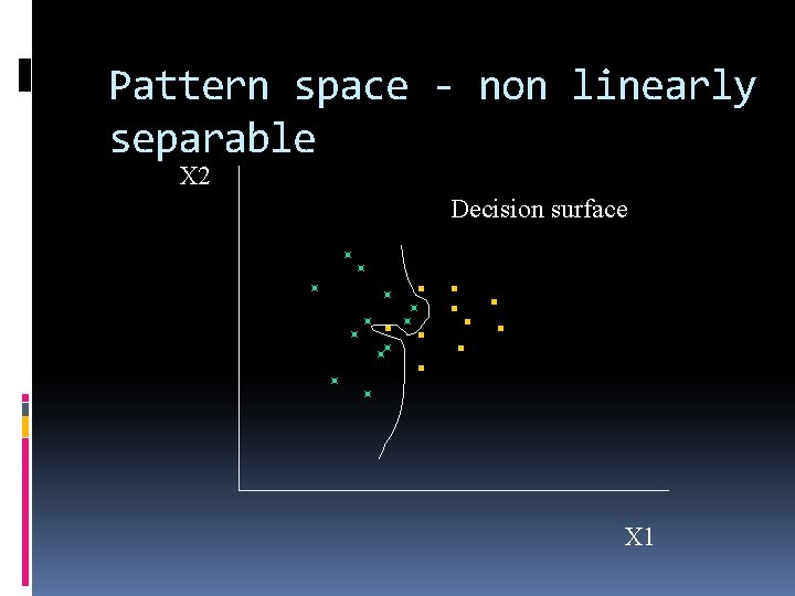
Non-linearly separable problems If a problem is not linearly separable, then it is impossible to divide the pattern space into two regions A network of neurons is needed

Pattern space - non linearly separable X 2 Decision surface X 1

The multi-layered perceptron (MLP)

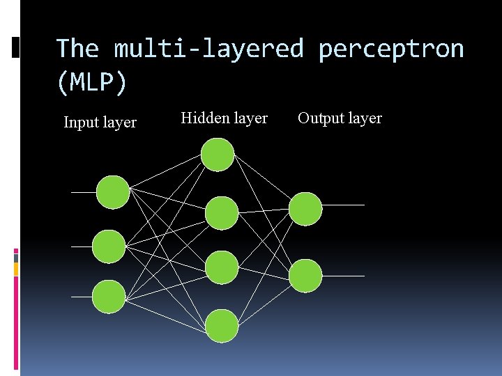
The multi-layered perceptron (MLP) Input layer Hidden layer Output layer

Complex decision surface The MLP has the ability to emulate any function using one hidden layer with a sigmoid function, and a linear output layer A 3 -layered network can therefore produce any complex decision surface However, the number of neurons in the hidden layer cannot be calculated

Network architecture All neurons in one layer are connected to all neurons in the next layer The network is a feedforward network, so all data flows from the input to the output The architecture of the network shown is described as 3: 4: 2 All neurons in the hidden and output layers have a bias connection

Input layer Receives all of the inputs Number of neurons equals the number of inputs Does no processing Connects to all the neurons in the hidden layer

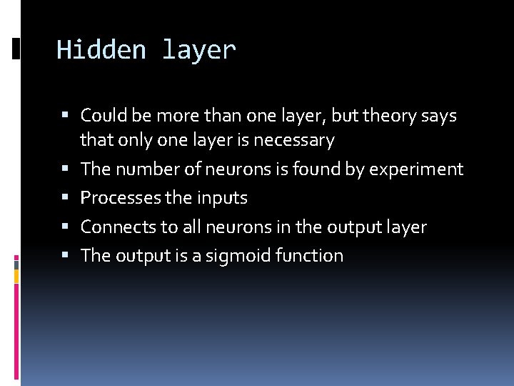
Hidden layer Could be more than one layer, but theory says that only one layer is necessary The number of neurons is found by experiment Processes the inputs Connects to all neurons in the output layer The output is a sigmoid function

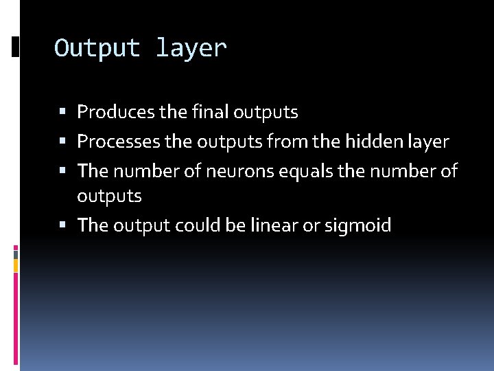
Output layer Produces the final outputs Processes the outputs from the hidden layer The number of neurons equals the number of outputs The output could be linear or sigmoid

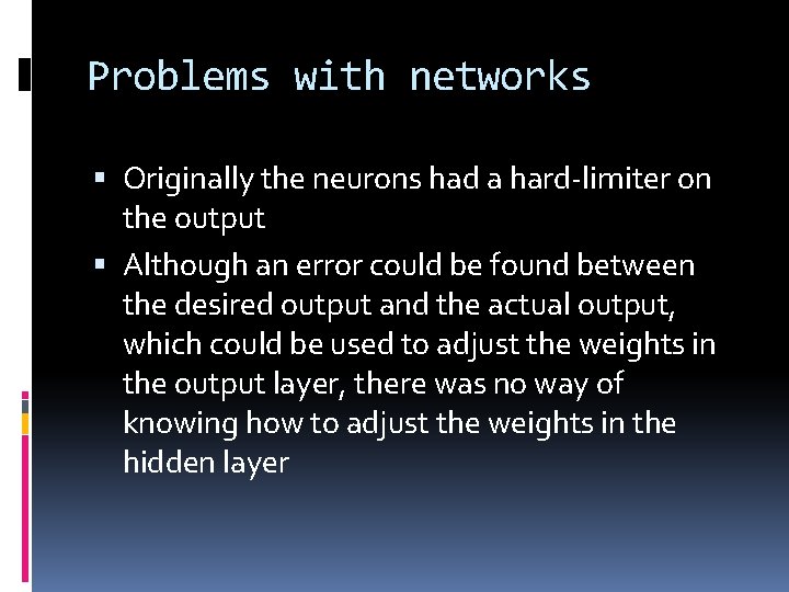
Problems with networks Originally the neurons had a hard-limiter on the output Although an error could be found between the desired output and the actual output, which could be used to adjust the weights in the output layer, there was no way of knowing how to adjust the weights in the hidden layer

The invention of backpropagation By introducing a smoothly changing output function, it was possible to calculate an error that could be used to adjust the weights in the hidden layer(s)

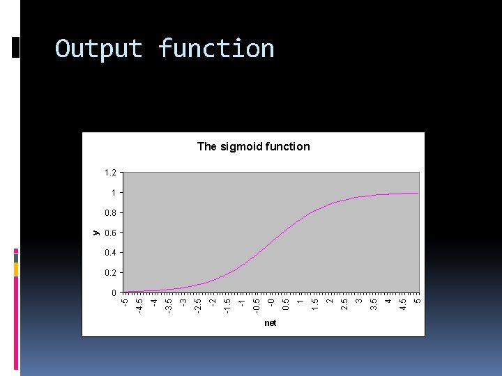
Output function The sigmoid function 1. 2 1 0. 6 0. 4 0. 2 net 5 4 3. 5 3 2. 5 2 1. 5 1 0. 5 -0 -0. 5 -1 -1. 5 -2 -2. 5 -3 -3. 5 -4 -4. 5 0 -5 y 0. 8

Sigmoid function The sigmoid function goes smoothly from 0 to 1 as net increases The value of y when net=0 is 0. 5 When net is negative, y is between 0 and 0. 5 When net is positive, y is between 0. 5 and 1. 0

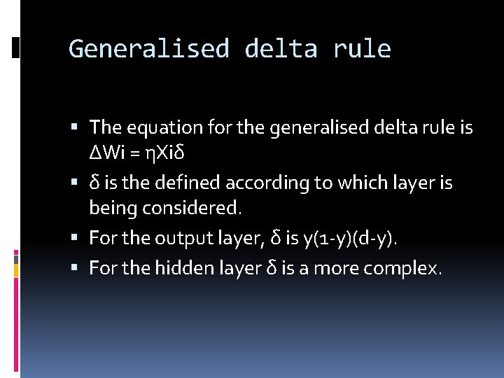
Back-propagation The method of training is called the backpropagation of errors The algorithm is an extension of the delta rule, called the generalised delta rule

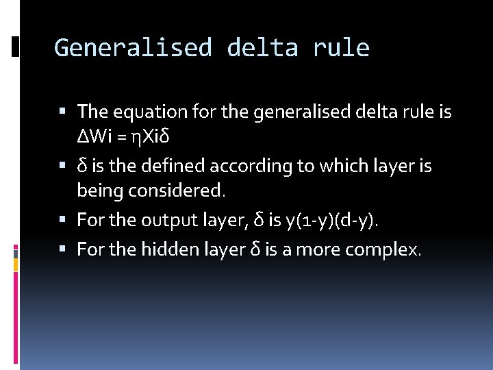
Generalised delta rule The equation for the generalised delta rule is ΔWi = ηXiδ δ is the defined according to which layer is being considered. For the output layer, δ is y(1 -y)(d-y). For the hidden layer δ is a more complex.

Training a network Example: The problem could not be implemented on a single layer - nonlinearly separable A 3 layer MLP was tried with 2 neurons in the hidden layer - which trained With 1 neuron in the hidden layer it failed to train

The hidden neurons

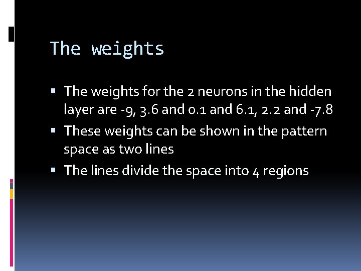
The weights for the 2 neurons in the hidden layer are -9, 3. 6 and 0. 1 and 6. 1, 2. 2 and -7. 8 These weights can be shown in the pattern space as two lines The lines divide the space into 4 regions

Training and Testing

Starting with a data set, the first step is to divide the data into a training set and a test set Use the training set to adjust the weights until the error is acceptably low Test the network using the test set, and see how many it gets right

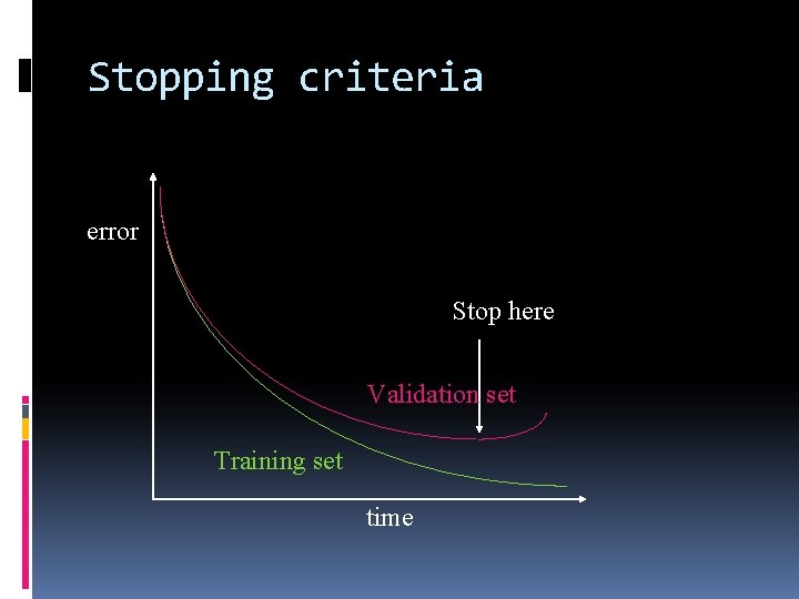
A better approach Critics of this standard approach have pointed out that training to a low error can sometimes cause “overfitting”, where the network performs well on the training data but poorly on the test data The alternative is to divide the data into three sets, the extra one being the validation set

Validation set During training, the training data is used to adjust the weights At each iteration, the validation/test data is also passed through the network and the error recorded but the weights are not adjusted The training stops when the error for the validation/test set starts to increase

Stopping criteria error Stop here Validation set Training set time

The multi-layered perceptron (MLP) and Backpropogation

Architecture Input layer Hidden layer Output layer

Back-propagation The method of training is called the backpropagation of errors The algorithm is an extension of the delta rule, called the generalised delta rule

Generalised delta rule The equation for the generalised delta rule is ΔWi = ηXiδ δ is the defined according to which layer is being considered. For the output layer, δ is y(1 -y)(d-y). For the hidden layer δ is a more complex.

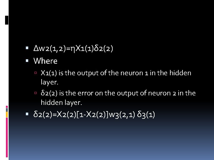
Hidden Layer We have to deal with the error from the output layer being feedbackwards to the hidden layer. Lets look at example the weight w 2(1, 2) Which is the weight connecting neuron 1 in the input layer with neuron 2 in the hidden layer.

Δw 2(1, 2)=ηX 1(1)δ 2(2) Where X 1(1) is the output of the neuron 1 in the hidden layer. δ 2(2) is the error on the output of neuron 2 in the hidden layer. δ 2(2)=X 2(2)[1 -X 2(2)]w 3(2, 1) δ 3(1)

δ 3(1) = y(1 -y)(d-y) =x 3(1)[1 -x 3(1)][d-x 3(1)] So we start with the error at the output and use this result to ripple backwards altering the weights.

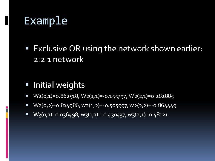
Example Exclusive OR using the network shown earlier: 2: 2: 1 network Initial weights W 2(0, 1)=0. 862518, W 2(1, 1)=-0. 155797, W 2(2, 1)=0. 282885 W 2(0, 2)=0. 834986, w 2(1, 2)=-0. 505997, w 2(2, 2)=-0. 864449 W 3(0, 1)=0. 036498, w 3(1, 1)=-0. 430437, w 3(2, 1)=0. 48121

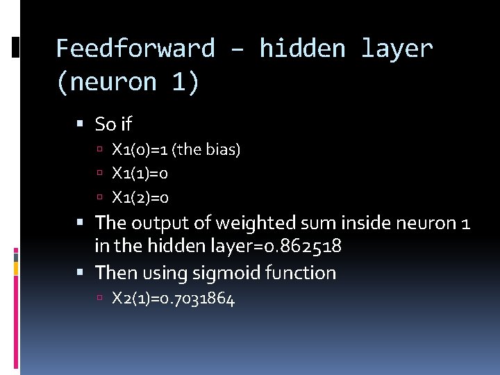
Feedforward – hidden layer (neuron 1) So if X 1(0)=1 (the bias) X 1(1)=0 X 1(2)=0 The output of weighted sum inside neuron 1 in the hidden layer=0. 862518 Then using sigmoid function X 2(1)=0. 7031864

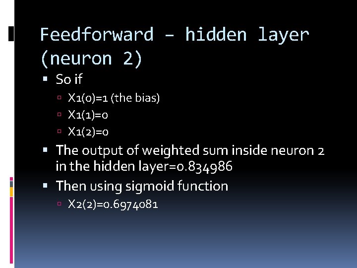
Feedforward – hidden layer (neuron 2) So if X 1(0)=1 (the bias) X 1(1)=0 X 1(2)=0 The output of weighted sum inside neuron 2 in the hidden layer=0. 834986 Then using sigmoid function X 2(2)=0. 6974081

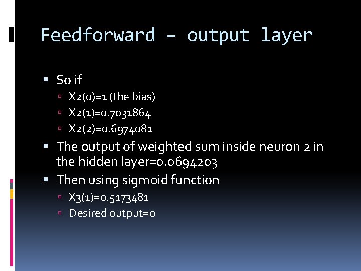
Feedforward – output layer So if X 2(0)=1 (the bias) X 2(1)=0. 7031864 X 2(2)=0. 6974081 The output of weighted sum inside neuron 2 in the hidden layer=0. 0694203 Then using sigmoid function X 3(1)=0. 5173481 Desired output=0

δ 3(1)=x 3(1)[1 -x 3(1)][d-x 3(1)] =-0. 1291812 δ 2(1)=X 2(1)[1 -X 2(1)]w 3(1, 1) δ 3(1)=0. 0116054 δ 2(2)=X 2(2)[1 -X 2(2)]w 3(2, 1) δ 3(1)=-0. 0131183 Now we can use the delta rule to calculate the change in the weights ΔWi = ηXiδ

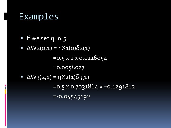
Examples If we set η=0. 5 ΔW 2(0, 1) = ηX 1(0)δ 2(1) =0. 5 x 1 x 0. 0116054 =0. 0058027 ΔW 3(2, 1) = ηX 2(1)δ 3(1) =0. 5 x 0. 7031864 x – 0. 1291812 =-0. 04545192

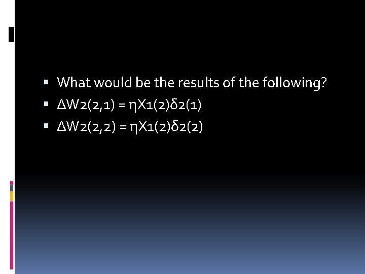
What would be the results of the following? ΔW 2(2, 1) = ηX 1(2)δ 2(1) ΔW 2(2, 2) = ηX 1(2)δ 2(2)

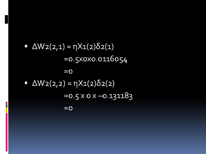
ΔW 2(2, 1) = ηX 1(2)δ 2(1) =0. 5 x 0 x 0. 0116054 =0 ΔW 2(2, 2) = ηX 1(2)δ 2(2) =0. 5 x 0 x – 0. 131183 =0

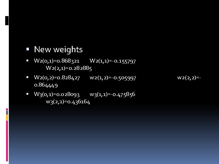
New weights W 2(0, 1)=0. 868321 W 2(1, 1)=-0. 155797 W 2(2, 1)=0. 282885 W 2(0, 2)=0. 828427 0. 864449 w 2(1, 2)=-0. 505997 W 3(0, 1)=0. 028093 w 3(1, 1)=-0. 475856 w 3(2, 1)=0. 436164 w 2(2, 2)=-