Snakes Active Contours Introduction Parametric active contours A

Snakes: Active Contours

Introduction

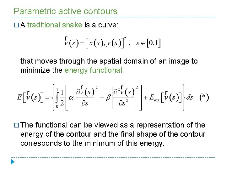
Parametric active contours �A traditional snake is a curve: that moves through the spatial domain of an image to minimize the energy functional: � The functional can be viewed as a representation of the energy of the contour and the final shape of the contour corresponds to the minimum of this energy.

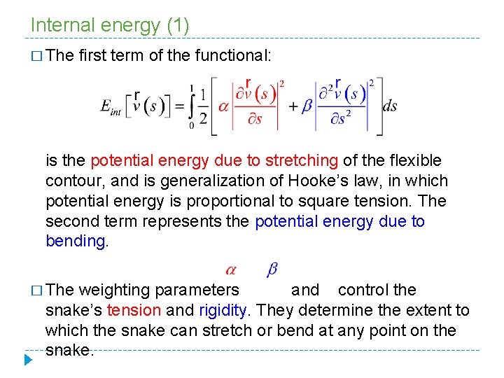
Internal energy (1) � The first term of the functional: is the potential energy due to stretching of the flexible contour, and is generalization of Hooke’s law, in which potential energy is proportional to square tension. The second term represents the potential energy due to bending. � The weighting parameters and control the snake’s tension and rigidity. They determine the extent to which the snake can stretch or bend at any point on the snake.

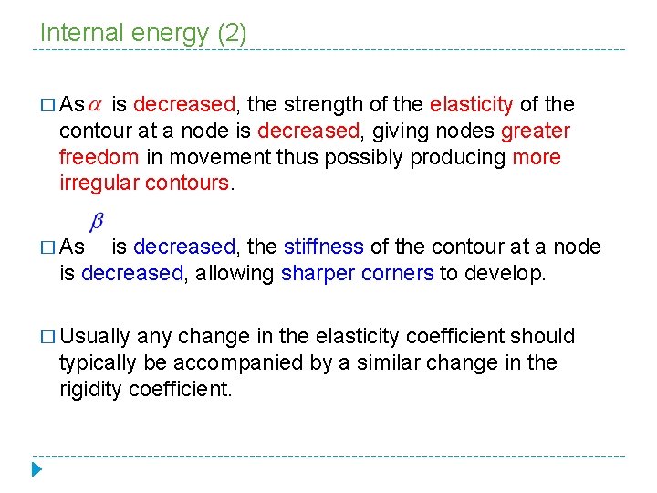
Internal energy (2) � As is decreased, the strength of the elasticity of the contour at a node is decreased, giving nodes greater freedom in movement thus possibly producing more irregular contours. � As is decreased, the stiffness of the contour at a node is decreased, allowing sharper corners to develop. � Usually any change in the elasticity coefficient should typically be accompanied by a similar change in the rigidity coefficient.

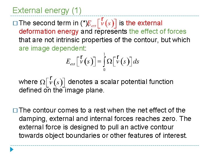
External energy (1) � The second term in (*), is the external deformation energy and represents the effect of forces that are not intrinsic properties of the contour, but which are image dependent: where denotes a scalar potential function defined on the image plane. � The contour comes to a rest when the net effect of the damping, external and internal forces reaches zero. The external force is designed to pull an active contour towards object boundaries or other features of interest.

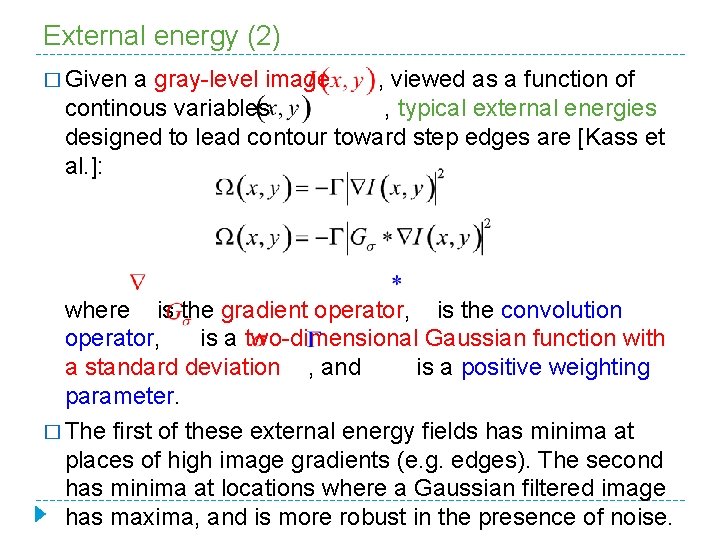
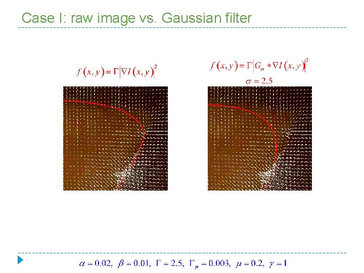
External energy (2) � Given a gray-level image , viewed as a function of continous variables , typical external energies designed to lead contour toward step edges are [Kass et al. ]: where is the gradient operator, is the convolution operator, is a two-dimensional Gaussian function with a standard deviation , and is a positive weighting parameter. � The first of these external energy fields has minima at places of high image gradients (e. g. edges). The second has minima at locations where a Gaussian filtered image has maxima, and is more robust in the presence of noise.

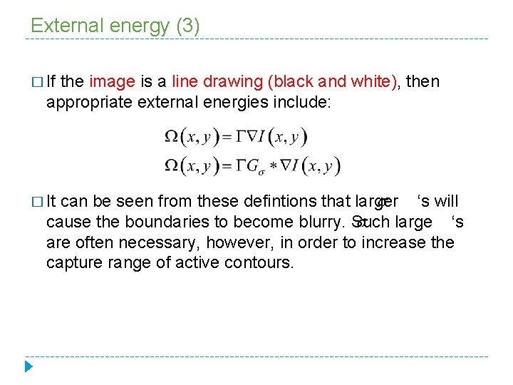
External energy (3) � If the image is a line drawing (black and white), then appropriate external energies include: � It can be seen from these defintions that larger ‘s will cause the boundaries to become blurry. Such large ‘s are often necessary, however, in order to increase the capture range of active contours.

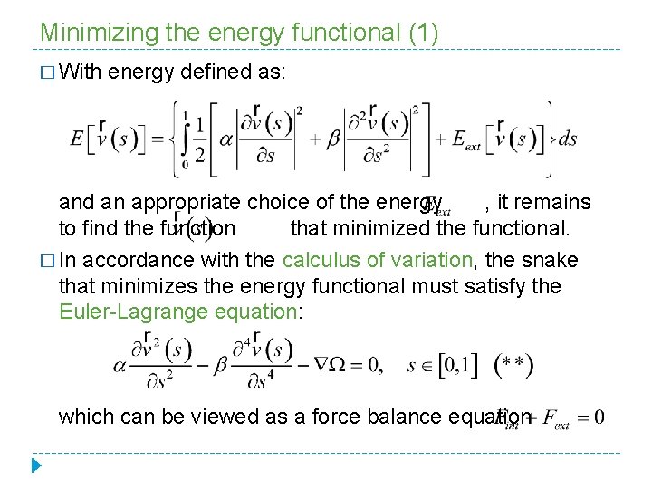
Minimizing the energy functional (1) � With energy defined as: and an appropriate choice of the energy , it remains to find the function that minimized the functional. � In accordance with the calculus of variation, the snake that minimizes the energy functional must satisfy the Euler-Lagrange equation: which can be viewed as a force balance equation

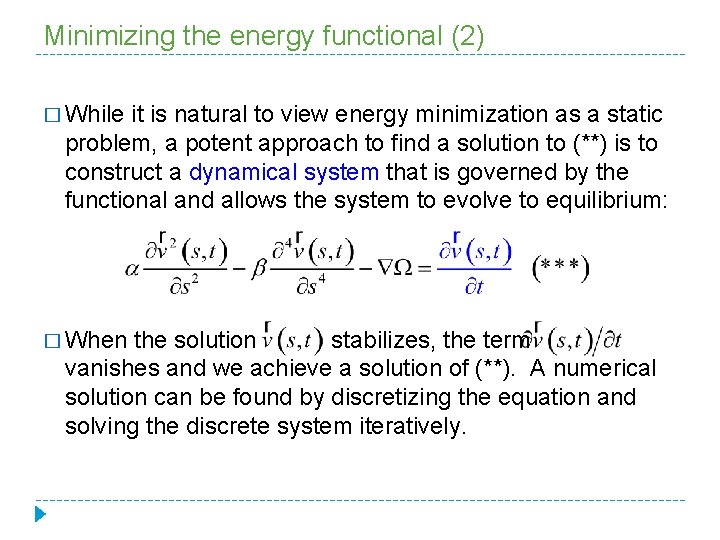
Minimizing the energy functional (2) � While it is natural to view energy minimization as a static problem, a potent approach to find a solution to (**) is to construct a dynamical system that is governed by the functional and allows the system to evolve to equilibrium: � When the solution stabilizes, the term vanishes and we achieve a solution of (**). A numerical solution can be found by discretizing the equation and solving the discrete system iteratively.

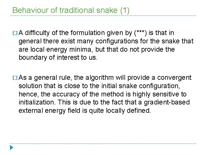
Behaviour of traditional snake (1) �A difficulty of the formulation given by (***) is that in general there exist many configurations for the snake that are local energy minima, but that do not provide the boundary of interest to us. � As a general rule, the algorithm will provide a convergent solution that is close to the initial snake configuration, hence, the accuracy of the method is highly sensitive to initialization. This is due to the fact that a gradient-based external energy field is quite locally defined.

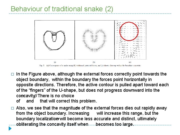
Behaviour of traditional snake (2) � In the Figure above, although the external forces correctly point towards the object boundary, within the boundary the forces point horizontally in opposite directions. Therefore, the active contour is pulled apart toward each of the “fingers” of the U-shape, but does not progress downward into the concavity. There is no choice of and that will correct this problem. � Also, we see that the magnitude of the external forces dies out rapidly away from the object boundary. Increasing will increase this range, but the boundary localization will become less accurate and distinct, ultimately obliterating the concavity itself when becomes too large.

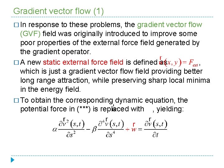
Gradient vector flow (1) � In response to these problems, the gradient vector flow (GVF) field was originally introduced to improve some poor properties of the external force field generated by the gradient operator. � A new static external force field is defined as , which is just a gradient vector flow field providing better long range attraction, while preserving sharp local minima in the energy field. � To obtain the corresponding dynamic equation, the potential force in (***) is replaced with , yielding:

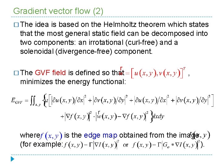
Gradient vector flow (2) � The idea is based on the Helmholtz theorem which states that the most general static field can be decomposed into two components: an irrotational (curl-free) and a solenoidal (divergence-free) component. � The GVF field is defined so that minimizes the energy functional: , where is the edge map obtained from the image (for example: ).

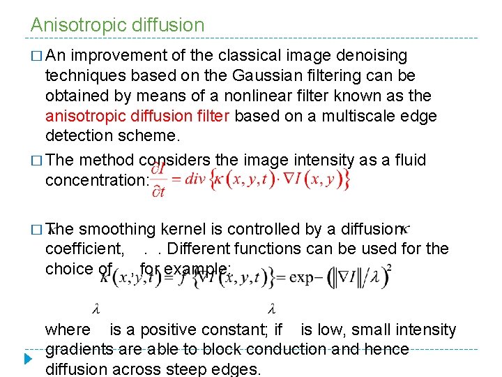
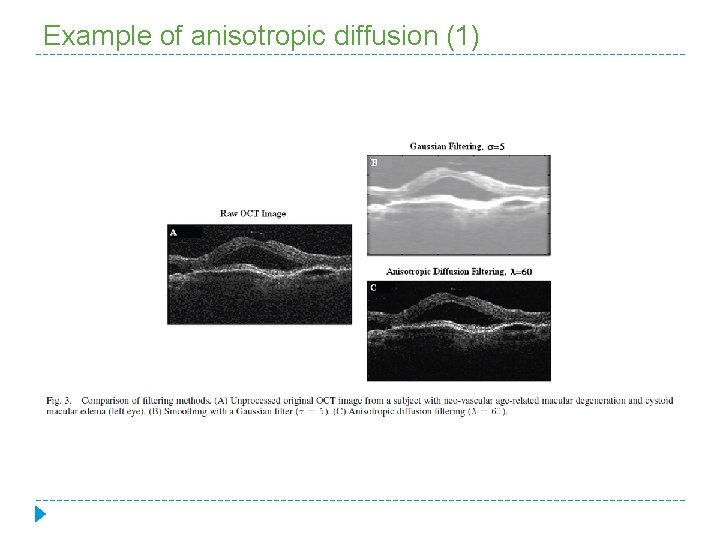
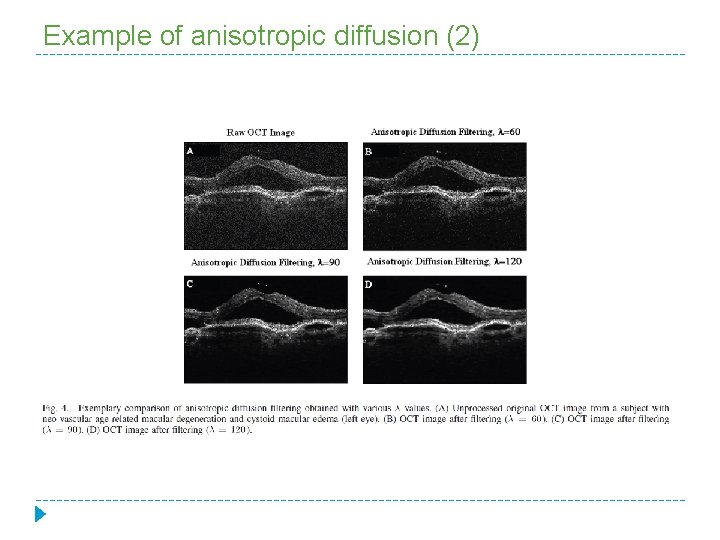
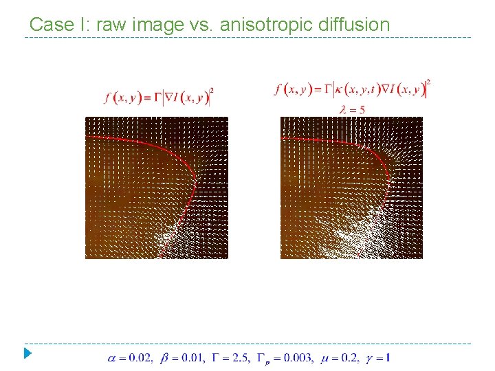
Anisotropic diffusion � An improvement of the classical image denoising techniques based on the Gaussian filtering can be obtained by means of a nonlinear filter known as the anisotropic diffusion filter based on a multiscale edge detection scheme. � The method considers the image intensity as a fluid concentration: � The smoothing kernel is controlled by a diffusion coefficient, . . Different functions can be used for the choice of , for example: where is a positive constant; if is low, small intensity gradients are able to block conduction and hence diffusion across steep edges.

Example of anisotropic diffusion (1)

Example of anisotropic diffusion (2)

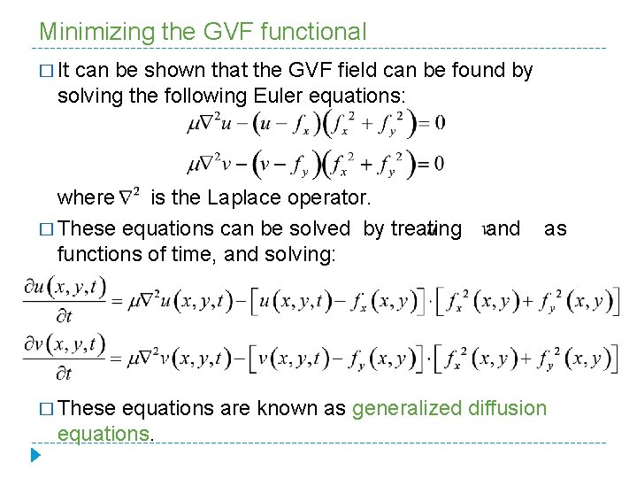
Minimizing the GVF functional � It can be shown that the GVF field can be found by solving the following Euler equations: where is the Laplace operator. � These equations can be solved by treating functions of time, and solving: � These and as equations are known as generalized diffusion equations.

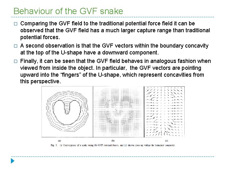
Behaviour of the GVF snake � Comparing the GVF field to the traditional potential force field it can be observed that the GVF field has a much larger capture range than traditional potential forces. � A second observation is that the GVF vectors within the boundary concavity at the top of the U-shape have a downward component. � Finally, it can be seen that the GVF field behaves in analogous fashion when viewed from inside the object. In particular, the GVF vectors are pointing upward into the “fingers” of the U-shape, which represent concavities from this perspective.

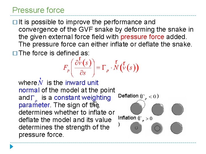
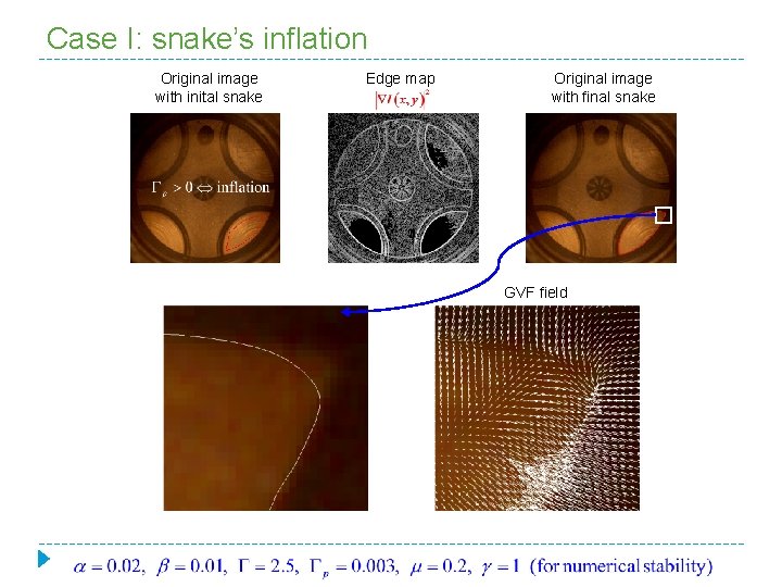
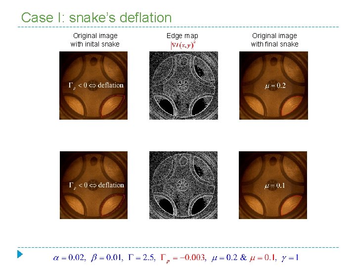
Pressure force � It is possible to improve the performance and convergence of the GVF snake by deforming the snake in the given external force field with pressure force added. The pressure force can either inflate or deflate the snake. � The force is defined as: where is the inward unit normal of the model at the point and is a constant weighting parameter. The sign of the determines whether to inflate or deflate the model and its value determines the strength of the pressure force. Deflation ( Inflation ( ) )

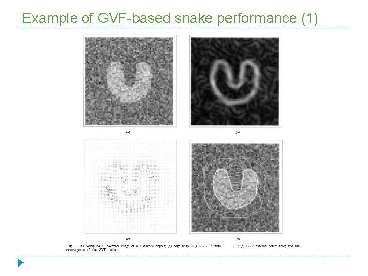
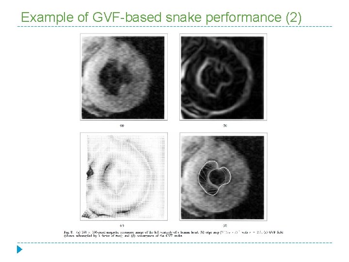
Example of GVF-based snake performance (1)

Example of GVF-based snake performance (2)

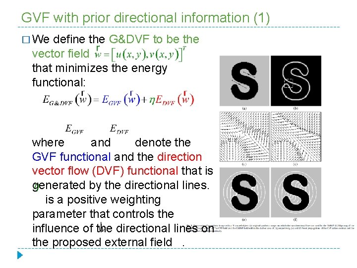
GVF with prior directional information (1) � We define the G&DVF to be the vector field that minimizes the energy functional: where and denote the GVF functional and the direction vector flow (DVF) functional that is generated by the directional lines. is a positive weighting parameter that controls the influence of the directional lines on the proposed external field.

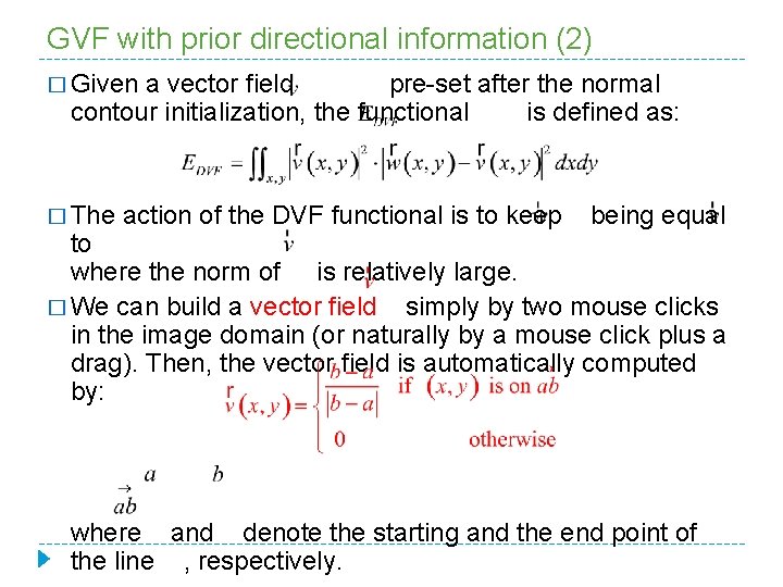
GVF with prior directional information (2) � Given a vector field pre-set after the normal contour initialization, the functional is defined as: � The action of the DVF functional is to keep being equal to where the norm of is relatively large. � We can build a vector field simply by two mouse clicks in the image domain (or naturally by a mouse click plus a drag). Then, the vector field is automatically computed by: where and denote the starting and the end point of the line , respectively.

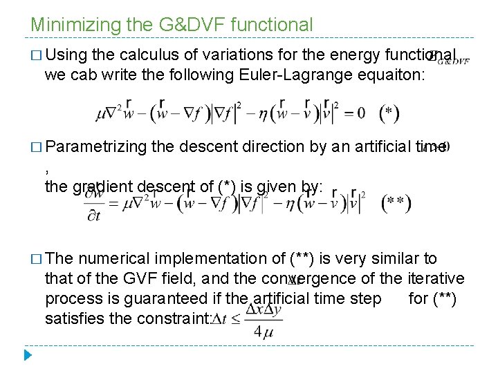
Minimizing the G&DVF functional � Using the calculus of variations for the energy functional we cab write the following Euler-Lagrange equaiton: � Parametrizing the descent direction by an artificial time , the gradient descent of (*) is given by: � The numerical implementation of (**) is very similar to that of the GVF field, and the convergence of the iterative process is guaranteed if the artificial time step for (**) satisfies the constraint:

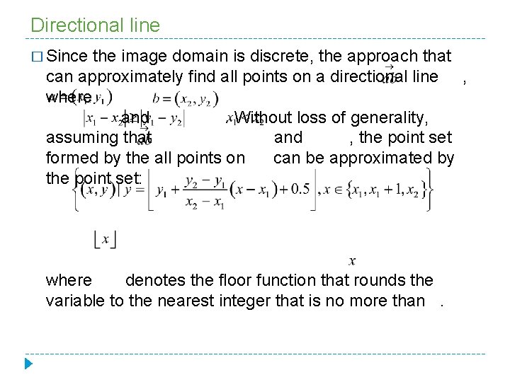
Directional line � Since the image domain is discrete, the approach that can approximately find all points on a directional line , where and. Without loss of generality, assuming that and , the point set formed by the all points on can be approximated by the point set: where denotes the floor function that rounds the variable to the nearest integer that is no more than.

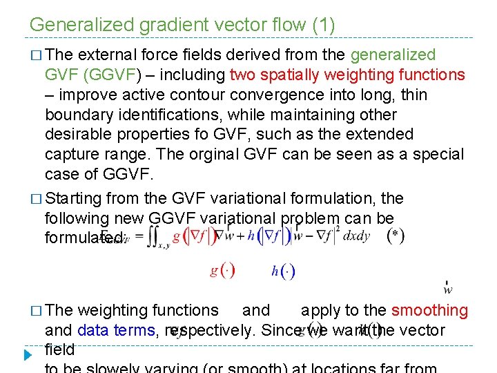
Generalized gradient vector flow (1) � The external force fields derived from the generalized GVF (GGVF) – including two spatially weighting functions – improve active contour convergence into long, thin boundary identifications, while maintaining other desirable properties fo GVF, such as the extended capture range. The orginal GVF can be seen as a special case of GGVF. � Starting from the GVF variational formulation, the following new GGVF variational problem can be formulated: � The weighting functions and apply to the smoothing and data terms, respectively. Since we want the vector field

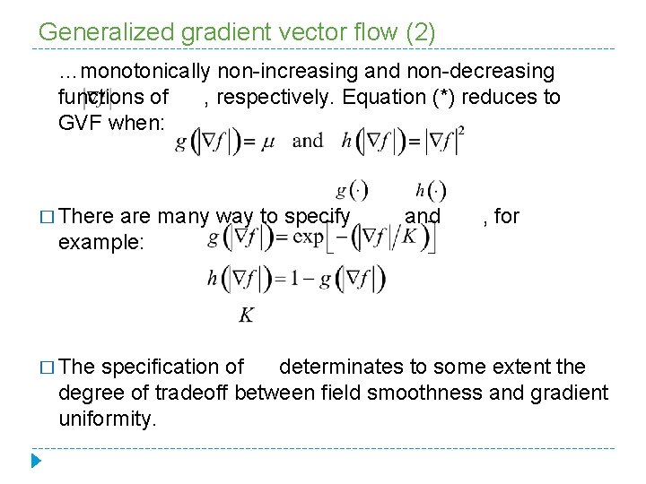
Generalized gradient vector flow (2) …monotonically non-increasing and non-decreasing functions of , respectively. Equation (*) reduces to GVF when: � There are many way to specify example: � The and , for specification of determinates to some extent the degree of tradeoff between field smoothness and gradient uniformity.

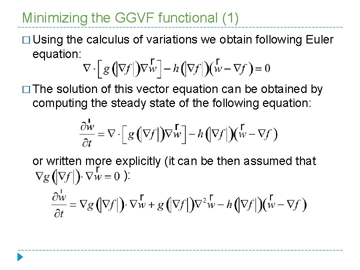
Minimizing the GGVF functional (1) � Using the calculus of variations we obtain following Euler equation: � The solution of this vector equation can be obtained by computing the steady state of the following equation: or written more explicitly (it can be then assumed that ):

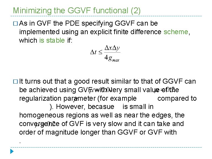
Minimizing the GGVF functional (2) � As in GVF the PDE specifying GGVF can be implemented using an explicit finite difference scheme, which is stable if: � It turns out that a good result similar to that of GGVF can be achieved using GVF with very small value of the regularization parameter (for example compared to ). However, becasue is small in homogeneous regions as well as near the edges, the convergence of GVF is very slow and it can take and order of magnitude longer than GGVF or GVF with.

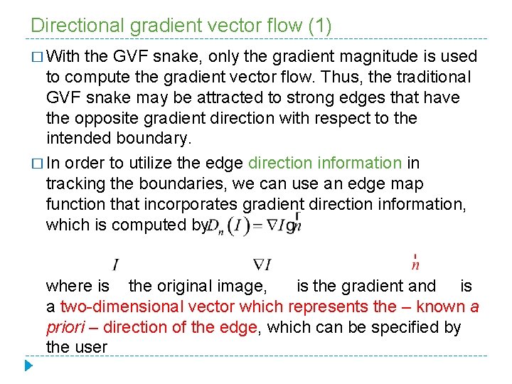
Directional gradient vector flow (1) � With the GVF snake, only the gradient magnitude is used to compute the gradient vector flow. Thus, the traditional GVF snake may be attracted to strong edges that have the opposite gradient direction with respect to the intended boundary. � In order to utilize the edge direction information in tracking the boundaries, we can use an edge map function that incorporates gradient direction information, which is computed by: where is the original image, is the gradient and is a two-dimensional vector which represents the – known a priori – direction of the edge, which can be specified by the user

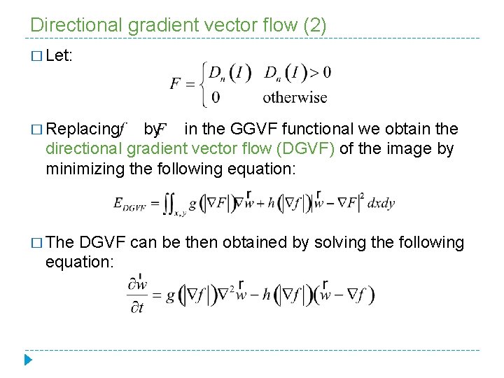
Directional gradient vector flow (2) � Let: � Replacing by in the GGVF functional we obtain the directional gradient vector flow (DGVF) of the image by minimizing the following equation: � The DGVF can be then obtained by solving the following equation:

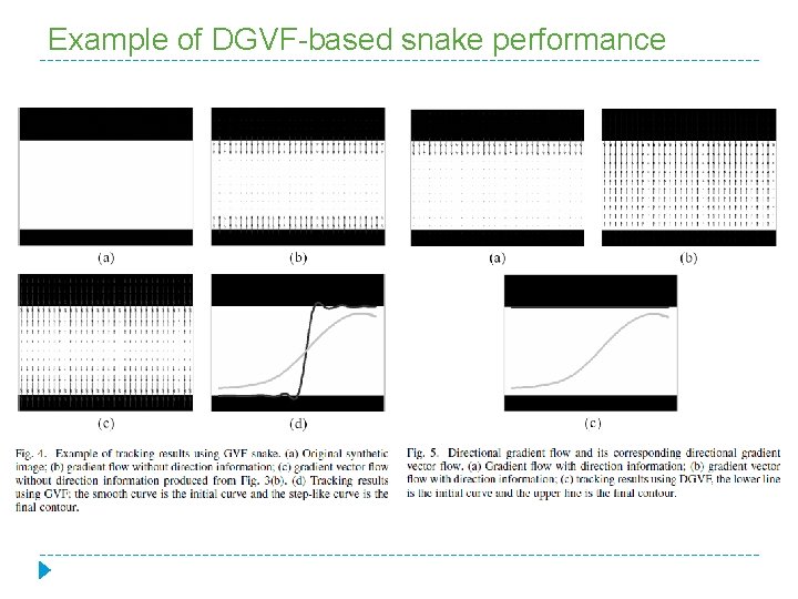
Example of DGVF-based snake performance

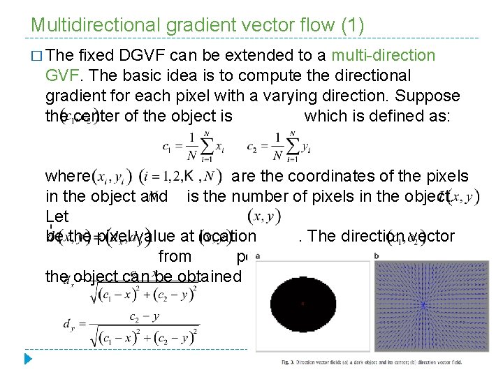
Multidirectional gradient vector flow (1) � The fixed DGVF can be extended to a multi-direction GVF. The basic idea is to compute the directional gradient for each pixel with a varying direction. Suppose the center of the object is which is defined as: where are the coordinates of the pixels in the object and is the number of pixels in the object. Let be the pixel value at location. The direction vector from pointing at the center of the object can be obtained using:

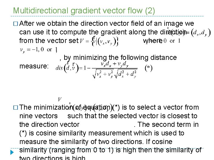
Multidirectional gradient vector flow (2) � After we obtain the direction vector field of an image we can use it to compute the gradient along the direction from the vector set where , , by minimizing the following distance measure: � The minimization of equation (*) is to select a vector from nine vectors such that the selected vector is closest to the direction vector. The second term in (*) is cosine similarity measurement which is used to measure the similarity of two directions. If cosine similarity (ranging from 0 to 1) is high then the similarity of

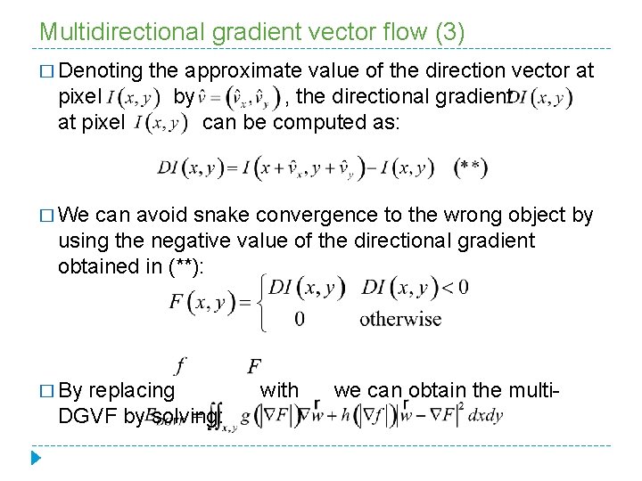
Multidirectional gradient vector flow (3) � Denoting pixel at pixel the approximate value of the direction vector at by , the directional gradient can be computed as: � We can avoid snake convergence to the wrong object by using the negative value of the directional gradient obtained in (**): � By replacing DGVF by solving: with we can obtain the multi-

Application to diesel engine images

Case I: snake’s inflation Original image with inital snake Edge map Original image with final snake GVF field

Case I: snake’s deflation Original image with inital snake Edge map Original image with final snake

Case I: raw image vs. Gaussian filter

Case I: raw image vs. anisotropic diffusion

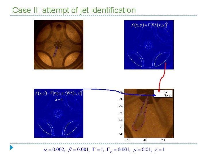
Case II: attempt of jet identification

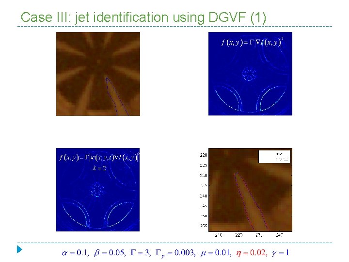
Case III: jet identification using DGVF (1)

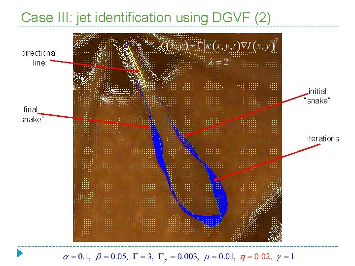
Case III: jet identification using DGVF (2) directional line initial “snake” final “snake” iterations