CH 4 Parametric Methods 4 1 Introduction Parametric

CH. 4: Parametric Methods 4. 1 Introduction Parametric methods are primarily rooted on the probability theory. Two subjects are considered here: (A) Parameter estimation – estimate parameters from given samples (B) Parametric classification – classification based on parameters 1

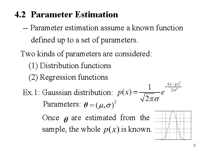
4. 2 Parameter Estimation -- Parameter estimation assume a known function defined up to a set of parameters. Two kinds of parameters are considered: (1) Distribution functions (2) Regression functions Ex. 1: Gaussian distribution: Parameters: Once are estimated from the sample, the whole is known. 2

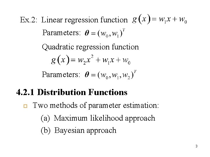
Ex. 2: Linear regression function Parameters: Quadratic regression function Parameters: 4. 2. 1 Distribution Functions Two methods of parameter estimation: (a) Maximum likelihood approach (b) Bayesian approach 3

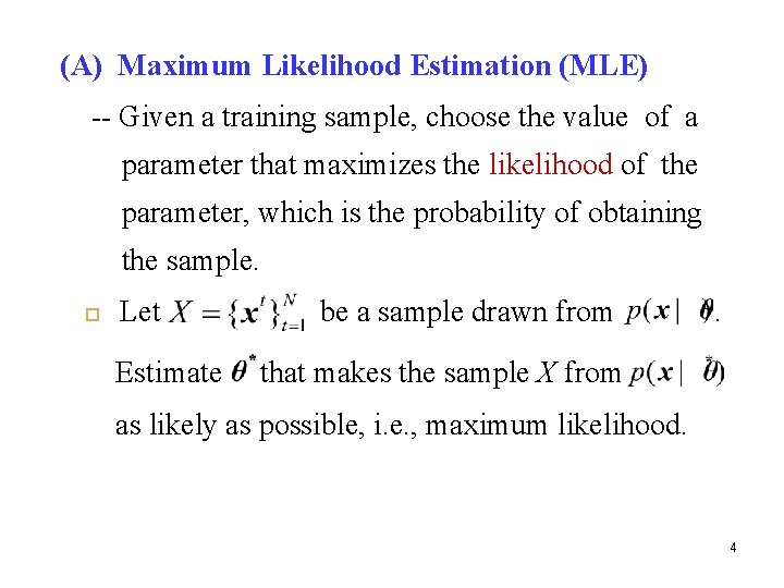
(A) Maximum Likelihood Estimation (MLE) -- Given a training sample, choose the value of a parameter that maximizes the likelihood of the parameter, which is the probability of obtaining the sample. Let Estimate be a sample drawn from . that makes the sample X from as likely as possible, i. e. , maximum likelihood. 4

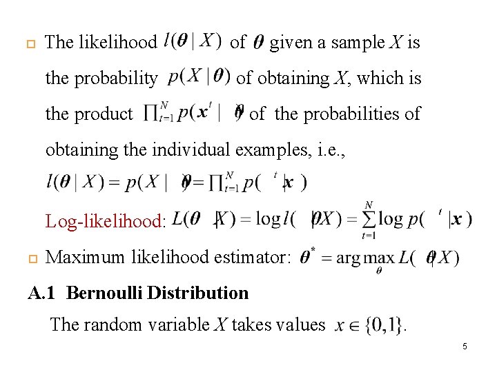
The likelihood the probability of given a sample X is of obtaining X, which is the product of the probabilities of obtaining the individual examples, i. e. , Log-likelihood: Maximum likelihood estimator: A. 1 Bernoulli Distribution The random variable X takes values . 5

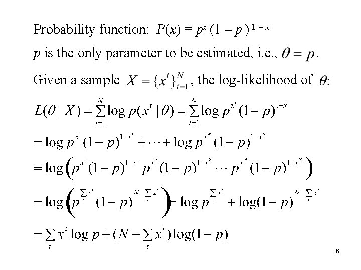
Probability function: P(x) = px (1 – p ) 1 – x p is the only parameter to be estimated, i. e. , Given a sample . , the log-likelihood of 6

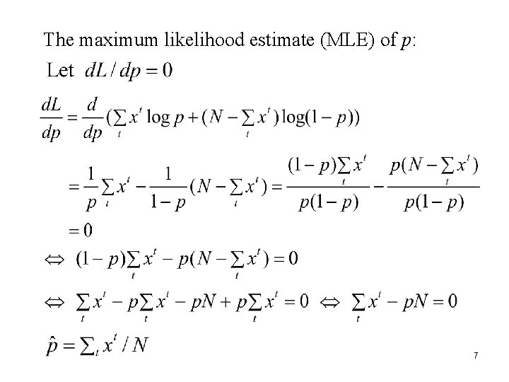
The maximum likelihood estimate (MLE) of p: 7

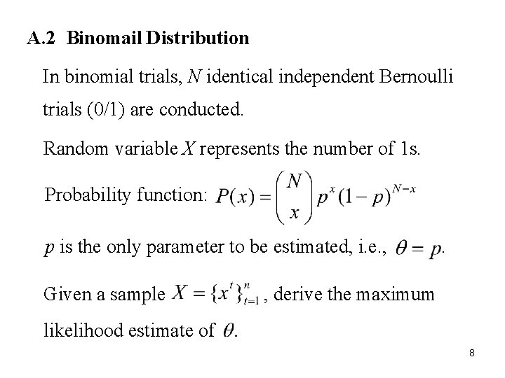
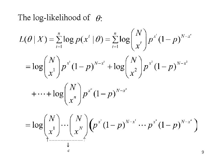
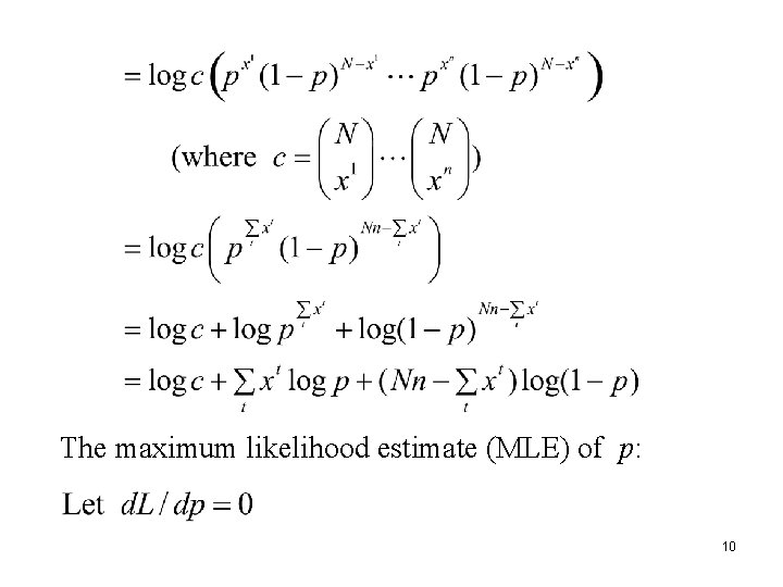
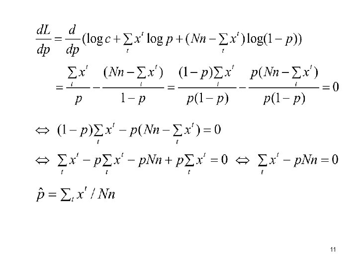
A. 2 Binomail Distribution In binomial trials, N identical independent Bernoulli trials (0/1) are conducted. Random variable X represents the number of 1 s. Probability function: p is the only parameter to be estimated, i. e. , Given a sample . , derive the maximum likelihood estimate of 8

The log-likelihood of 9

The maximum likelihood estimate (MLE) of p: 10

11

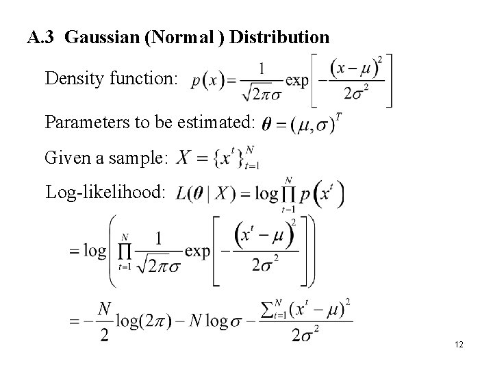
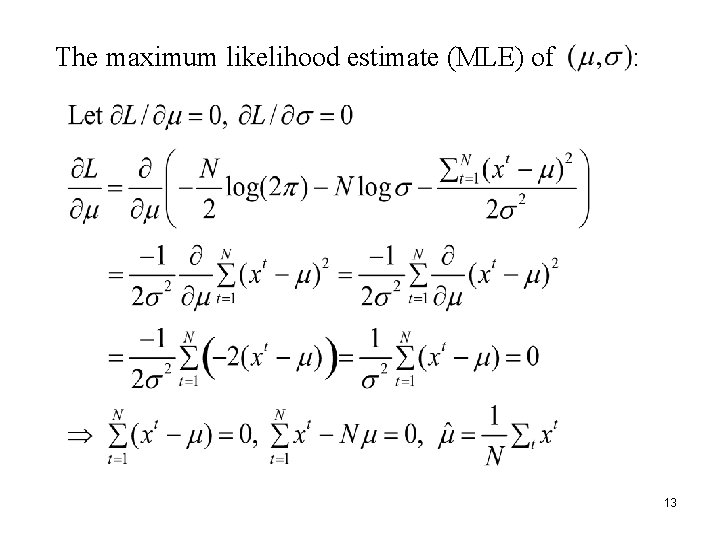
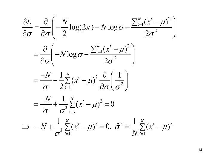
A. 3 Gaussian (Normal ) Distribution Density function: Parameters to be estimated: Given a sample: Log-likelihood: 12

The maximum likelihood estimate (MLE) of : 13

14

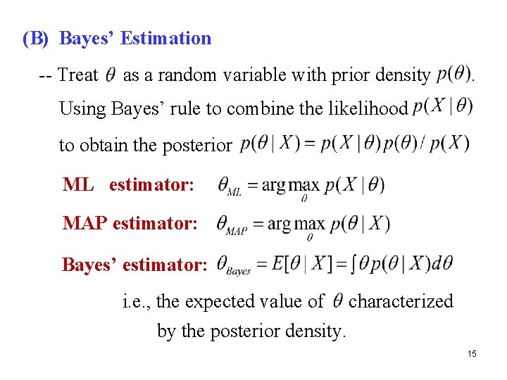
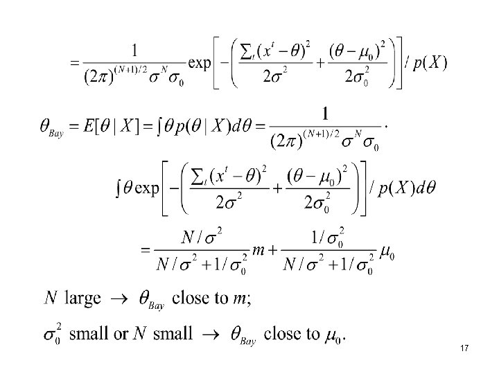
(B) Bayes’ Estimation -- Treat as a random variable with prior density . Using Bayes’ rule to combine the likelihood to obtain the posterior ML estimator: . MAP estimator: Bayes’ estimator: i. e. , the expected value of characterized by the posterior density. 15

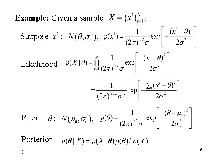
Example: Given a sample Suppose Likelihood: Prior: Posterior : 16

17

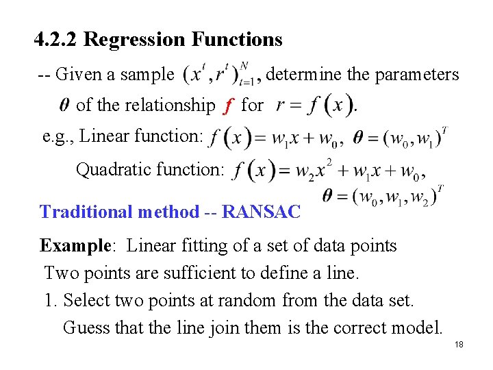
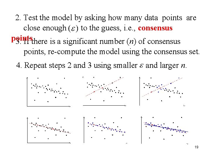
4. 2. 2 Regression Functions -- Given a sample determine the parameters of the relationship f for e. g. , Linear function: Quadratic function: Traditional method -- RANSAC Example: Linear fitting of a set of data points Two points are sufficient to define a line. 1. Select two points at random from the data set. Guess that the line join them is the correct model. 18

2. Test the model by asking how many data points are close enough to the guess, i. e. , consensus points. 3. If there is a significant number (n) of consensus points, re-compute the model using the consensus set. 4. Repeat steps 2 and 3 using smaller and larger n. 19

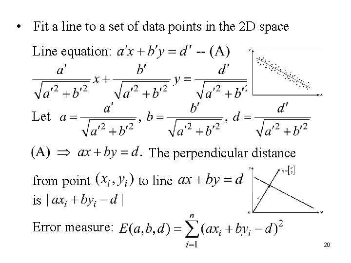
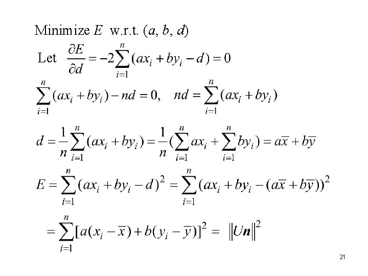
• Fit a line to a set of data points in the 2 D space Line equation: Let The perpendicular distance from point is to line Error measure: 20

Minimize E w. r. t. (a, b, d) Let 21

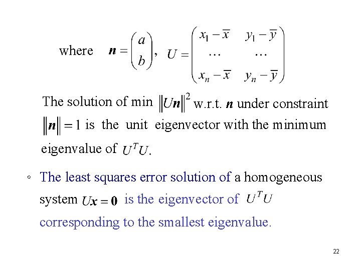
where The solution of min w. r. t. n under constraint is the unit eigenvector with the minimum eigenvalue of 。 The least squares error solution of a homogeneous system is the eigenvector of corresponding to the smallest eigenvalue. 22

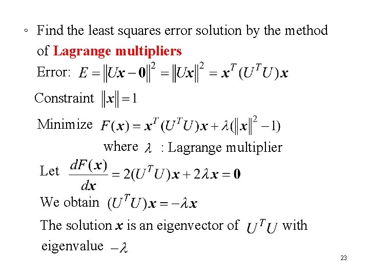
。 Find the least squares error solution by the method of Lagrange multipliers Error: Constraint Minimize where : Lagrange multiplier Let We obtain The solution x is an eigenvector of eigenvalue with 23

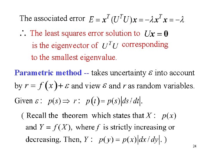
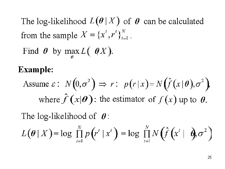
The associated error The least squares error solution to corresponding is the eigenvector of to the smallest eigenvalue. Parametric method -- takes uncertainty by and view into account and r as random variables. 24

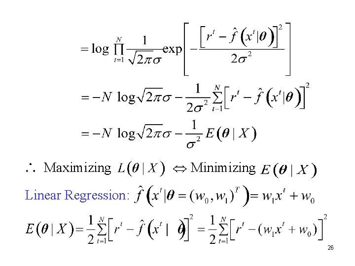
The log-likelihood of from the sample can be calculated . Example: where The log-likelihood of the estimator up to : 25

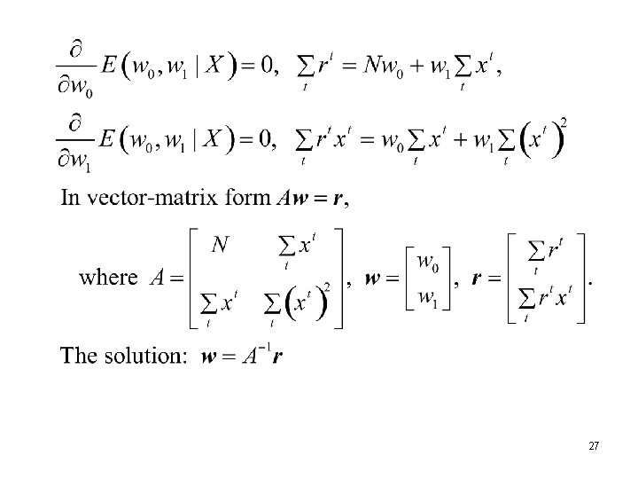
Maximizing Minimizing Linear Regression: 26

27

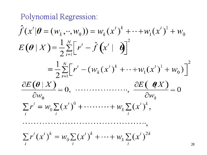
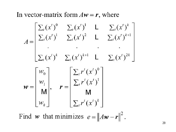
Polynomial Regression: 28

Find w that minimizes 29

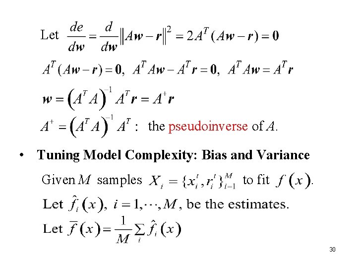
Let the pseudoinverse of A. • Tuning Model Complexity: Bias and Variance Given M samples to fit . 30

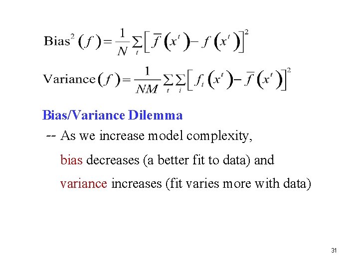
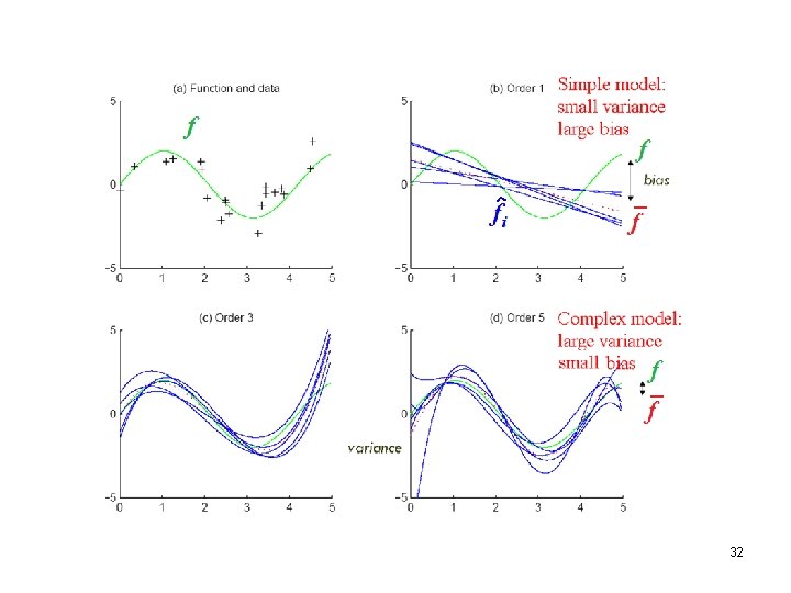
Bias/Variance Dilemma -- As we increase model complexity, bias decreases (a better fit to data) and variance increases (fit varies more with data) 31

32

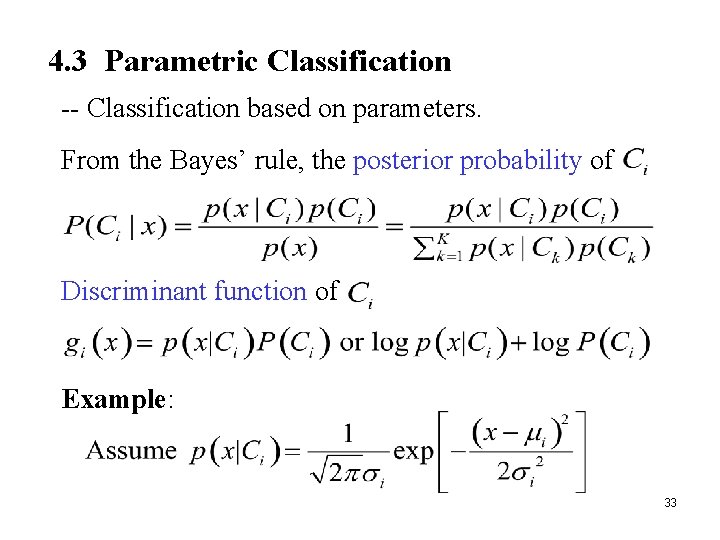
4. 3 Parametric Classification -- Classification based on parameters. From the Bayes’ rule, the posterior probability of Discriminant function of Example: 33

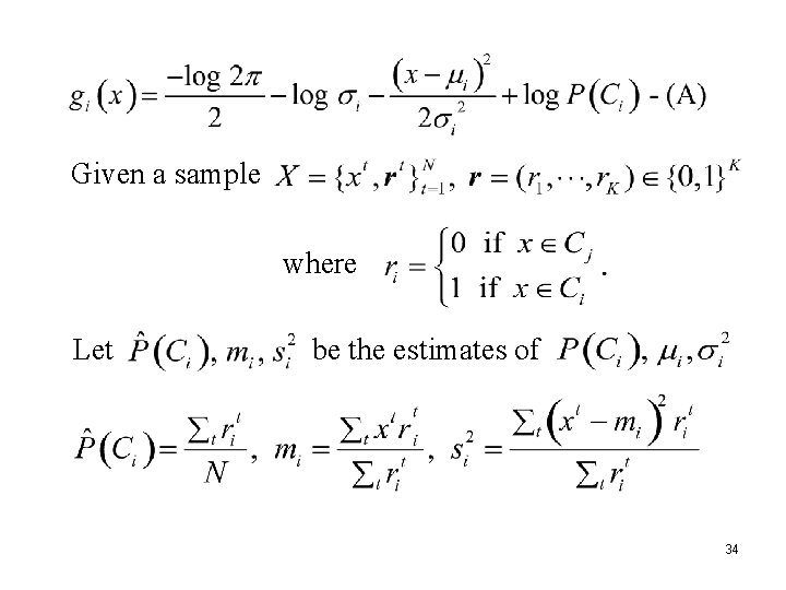
Given a sample where Let be the estimates of 34

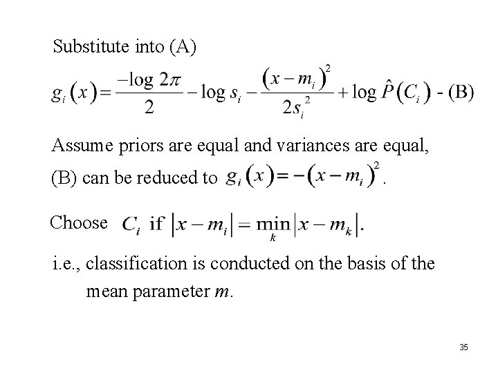
Substitute into (A) Assume priors are equal and variances are equal, (B) can be reduced to . Choose i. e. , classification is conducted on the basis of the mean parameter m. 35

Summary Parametric methods are primarily rooted on the probability theory. Two subjects are considered: (a) Parameter estimation (b) Parametric classification Parameter estimation assume a known function defined up to a set of parameters. Two kinds of parameters are considered: (i) Distribution functions (ii) Regression functions 36

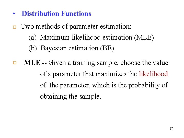
• Distribution Functions Two methods of parameter estimation: (a) Maximum likelihood estimation (MLE) (b) Bayesian estimation (BE) MLE -- Given a training sample, choose the value of a parameter that maximizes the likelihood of the parameter, which is the probability of obtaining the sample. 37

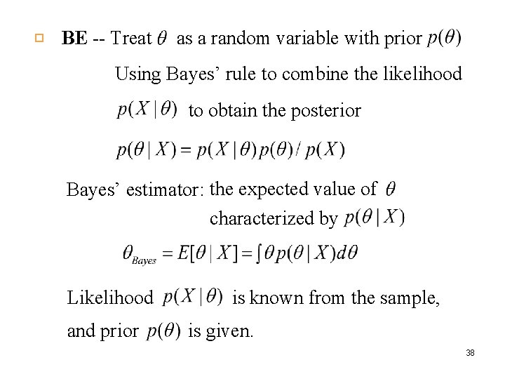
BE -- Treat as a random variable with prior Using Bayes’ rule to combine the likelihood to obtain the posterior Bayes’ estimator: the expected value of characterized by Likelihood and prior is known from the sample, is given. 38

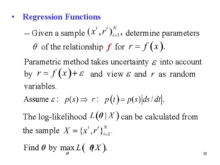
• Regression Functions -- Given a sample determine parameters of the relationship f for Parametric method takes uncertainty into account by and view and r as random variables. The log-likelihood the sample can be calculated from. 39

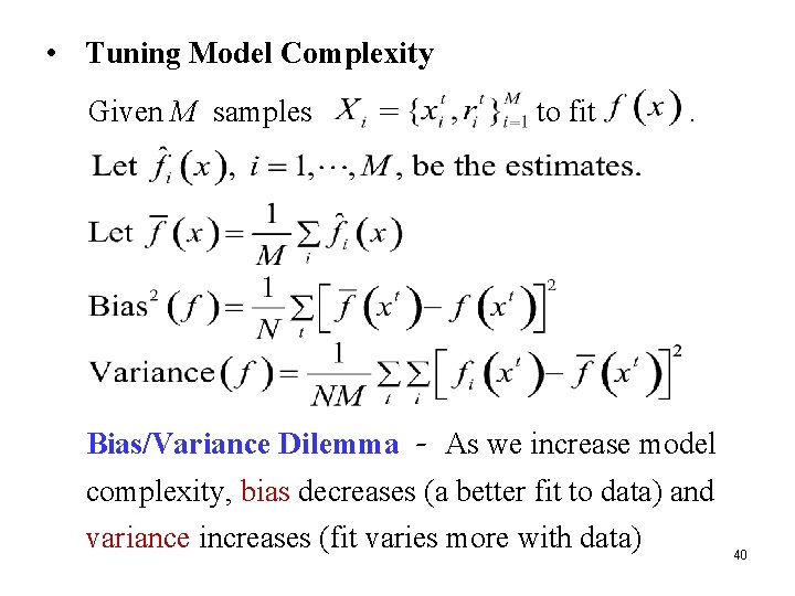
• Tuning Model Complexity Given M samples to fit . Bias/Variance Dilemma - As we increase model complexity, bias decreases (a better fit to data) and variance increases (fit varies more with data) 40