Parametric versus Nonparametric Statisticswhen to use them and

Parametric versus Nonparametric Statistics-when to use them and which is more powerful? Dr Mahmoud Alhussami

Parametric Assumptions Ø Ø Ø The observations must be independent. Dependent variable should be continuous (I/R) The observations must be drawn from normally distributed populations These populations must have the same variances. Equal variance (homogeneity of variance) The groups should be randomly drawn from normally distributed and independent populations e. g. Male X Female Nurse X Physician Manager X Staff NO OVER LAP

Parametric Assumptions The independent variable is categorical with two or more levels. q Distribution for the two or more independent variables is normal. q large variation = less likely to have sig t or F test = accepting null hypothesis (fail to reject) = Type II error = a threat to power Sending an innocent to jail for no significant reason q

Advantages of Parametric Techniques Ø They are more powerful and more flexible than nonparametric techniques. Ø They not only allow the researcher to study the effect of many independent variables on the dependent variable, but they also make possible the study of their interaction.

Nonparametric Methods Ø Ø Ø Most of the statistical methods referred to as parametric require the use of interval- or ratio-scaled data. Nonparametric methods are often the only way to analyze nominal or ordinal data and draw statistical conclusions. Nonparametric methods require no assumptions about the population probability distributions. Nonparametric methods are often called distributionfree methods. Nonparametric methods can be used with small samples

Nonparametric Methods Ø In general, for a statistical method to be classified as nonparametric, it must satisfy at least one of the following conditions. l l l The method can be used with nominal data. The method can be used with ordinal data. The method can be used with interval or ratio data when no assumption can be made about the population probability distribution.

Non Parametric Tests Ø Do not make as many assumptions about the distribution of the data as the t test. l l Do not require data to be Normal Good for data with outliers Ø Non-parametric tests based on ranks of the data l Work well for ordinal data (data that have a defined order, but for which averages may not make sense).

Nonparametric Methods Ø There is at least one nonparametric test equivalent to a parametric test Ø These tests fall into several categories 1. 2. 3. Tests of differences between groups (independent samples) Tests of differences between variables (dependent samples) Tests of relationships between variables

Advantages of Nonparametric Techniques Sometimes there is no parametric alternative to the use of nonparametric statistics. Ø Certain nonparametric test can be used to analyze nominal data. Ø Certain nonparametric test can be used to analyze ordinal data. Ø The computations on nonparametric statistics are usually less complicated than those for parametric statistics, particularly for small samples. Ø Probability statements obtained from most nonparametric tests are exact probabilities. Ø

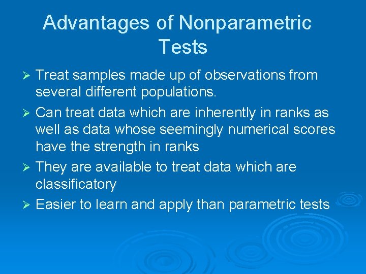
Advantages of Nonparametric Tests Treat samples made up of observations from several different populations. Ø Can treat data which are inherently in ranks as well as data whose seemingly numerical scores have the strength in ranks Ø They are available to treat data which are classificatory Ø Easier to learn and apply than parametric tests Ø

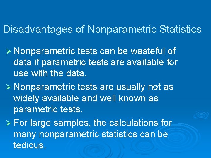
Disadvantages of Nonparametric Statistics Ø Nonparametric tests can be wasteful of data if parametric tests are available for use with the data. Ø Nonparametric tests are usually not as widely available and well known as parametric tests. Ø For large samples, the calculations for many nonparametric statistics can be tedious.

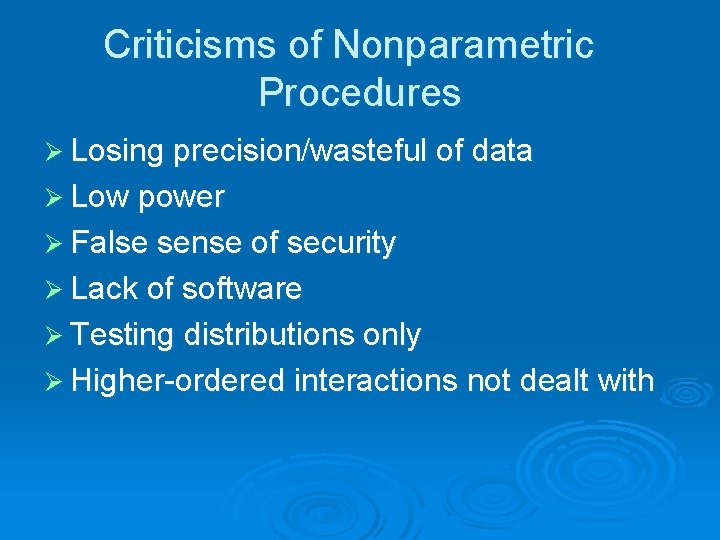
Criticisms of Nonparametric Procedures Ø Losing precision/wasteful of data Ø Low power Ø False sense of security Ø Lack of software Ø Testing distributions only Ø Higher-ordered interactions not dealt with

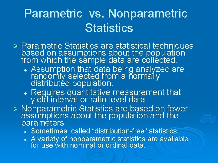
Parametric vs. Nonparametric Statistics Parametric Statistics are statistical techniques based on assumptions about the population from which the sample data are collected. l Assumption that data being analyzed are randomly selected from a normally distributed population. l Requires quantitative measurement that yield interval or ratio level data. Ø Nonparametric Statistics are based on fewer assumptions about the population and the parameters. Ø l l Sometimes called “distribution-free” statistics. A variety of nonparametric statistics are available for use with nominal or ordinal data.

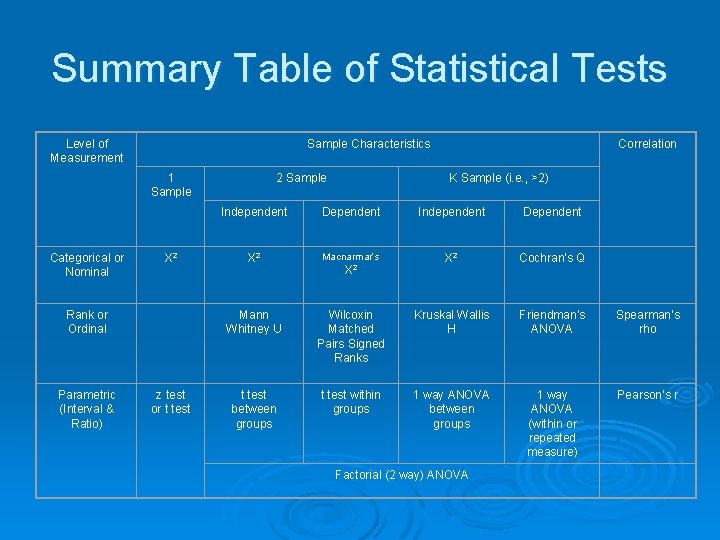
Summary Table of Statistical Tests Level of Measurement Correlation Sample Characteristics 1 Sample 2 Sample Independent K Sample (i. e. , >2) Dependent Independent Dependent Χ 2 Cochran’s Q Categorical or Nominal Χ 2 Macnarmar’s Rank or Ordinal Mann Whitney U Wilcoxin Matched Pairs Signed Ranks Kruskal Wallis H Friendman’s ANOVA Spearman’s rho Parametric (Interval & Ratio) z test or t test between groups t test within groups 1 way ANOVA between groups 1 way ANOVA (within or repeated measure) Pearson’s r Χ 2 Factorial (2 way) ANOVA

Chi-Square

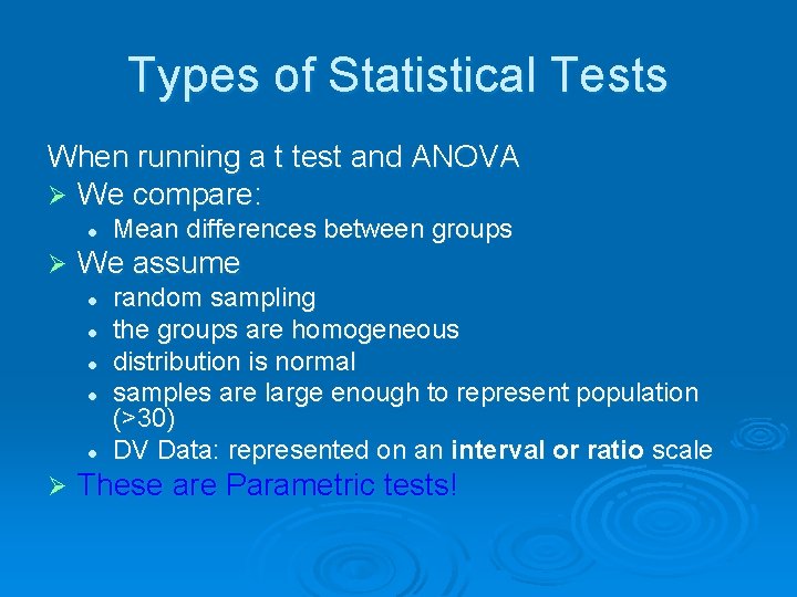
Types of Statistical Tests When running a t test and ANOVA Ø We compare: l Ø We assume l l l Ø Mean differences between groups random sampling the groups are homogeneous distribution is normal samples are large enough to represent population (>30) DV Data: represented on an interval or ratio scale These are Parametric tests!

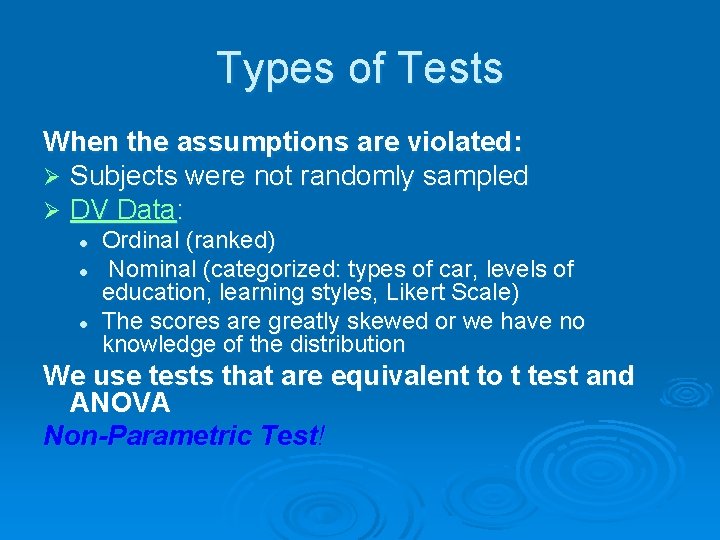
Types of Tests When the assumptions are violated: Ø Subjects were not randomly sampled Ø DV Data: l l l Ordinal (ranked) Nominal (categorized: types of car, levels of education, learning styles, Likert Scale) The scores are greatly skewed or we have no knowledge of the distribution We use tests that are equivalent to t test and ANOVA Non-Parametric Test!

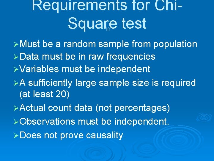
Requirements for Chi. Square test 18 ØMust be a random sample from population ØData must be in raw frequencies ØVariables must be independent ØA sufficiently large sample size is required (at least 20) ØActual count data (not percentages) ØObservations must be independent. ØDoes not prove causality.

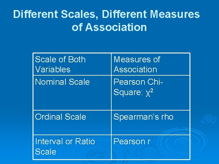
Different Scales, Different Measures of Association Scale of Both Variables Nominal Scale Measures of Association Pearson Chi. Square: χ2 Ordinal Scale Spearman’s rho Interval or Ratio Scale Pearson r

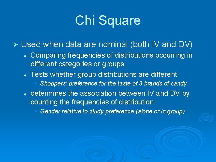
Chi Square Ø Used when data are nominal (both IV and DV) l l Comparing frequencies of distributions occurring in different categories or groups Tests whether group distributions are different • Shoppers’ preference for the taste of 3 brands of candy l determines the association between IV and DV by counting the frequencies of distribution • Gender relative to study preference (alone or in group)

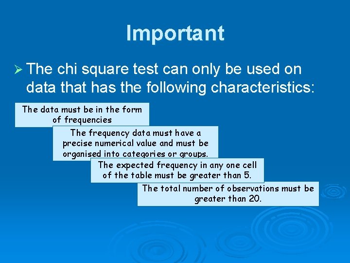
Important Ø The chi square test can only be used on data that has the following characteristics: The data must be in the form of frequencies The frequency data must have a precise numerical value and must be organised into categories or groups. The expected frequency in any one cell of the table must be greater than 5. The total number of observations must be greater than 20.

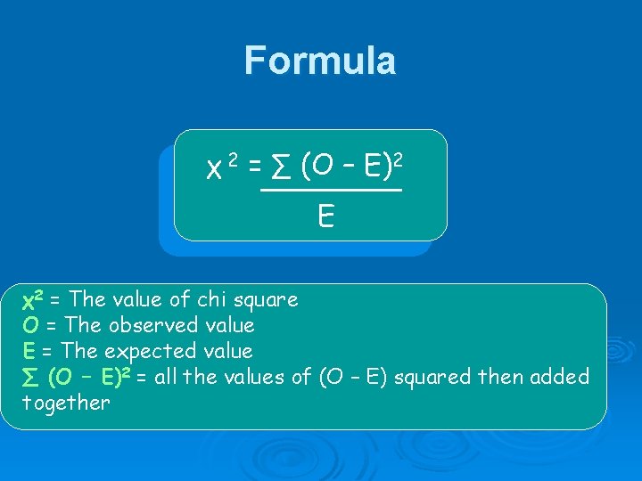
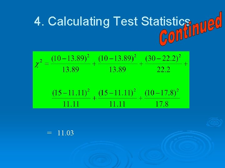
Formula χ 2 = ∑ (O – E)2 E χ2 = The value of chi square O = The observed value E = The expected value ∑ (O – E)2 = all the values of (O – E) squared then added together

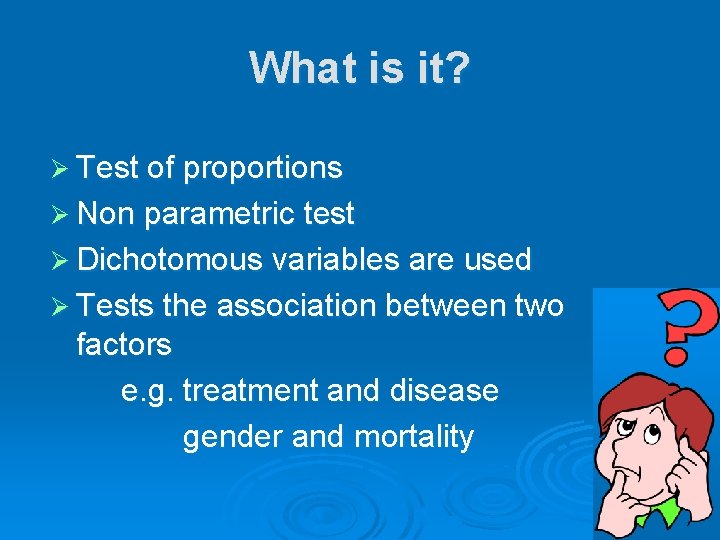
What is it? Ø Test of proportions Ø Non parametric test Ø Dichotomous variables are used Ø Tests the association between two factors e. g. treatment and disease gender and mortality

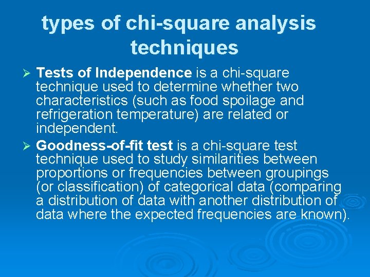
types of chi-square analysis techniques Tests of Independence is a chi-square technique used to determine whether two characteristics (such as food spoilage and refrigeration temperature) are related or independent. Ø Goodness-of-fit test is a chi-square test technique used to study similarities between proportions or frequencies between groupings (or classification) of categorical data (comparing a distribution of data with another distribution of data where the expected frequencies are known). Ø

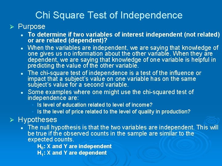
Chi Square Test of Independence Ø Purpose l l To determine if two variables of interest independent (not related) or are related (dependent)? When the variables are independent, we are saying that knowledge of one gives us no information about the other variable. When they are dependent, we are saying that knowledge of one variable is helpful in predicting the value of the other variable. The chi-square test of independence is a test of the influence or impact that a subject’s value on one variable has on the same subject’s value for a second variable. Some examples where one might use the chi-squared test of independence are: • Is level of education related to level of income? • Is the level of price related to the level of quality in production? Ø Hypotheses l The null hypothesis is that the two variables are independent. This will be true if the observed counts in the sample are similar to the expected counts. • H 0: X and Y are independent • H 1: X and Y are dependent

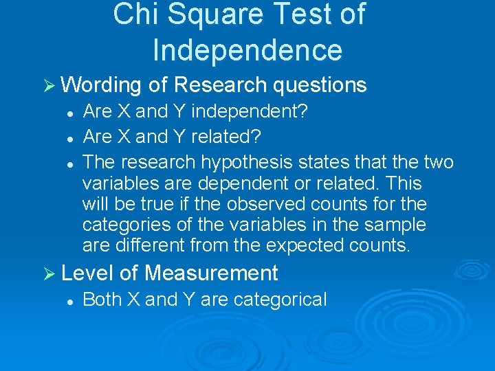
Chi Square Test of Independence Ø Wording of Research questions l l l Are X and Y independent? Are X and Y related? The research hypothesis states that the two variables are dependent or related. This will be true if the observed counts for the categories of the variables in the sample are different from the expected counts. Ø Level of Measurement l Both X and Y are categorical

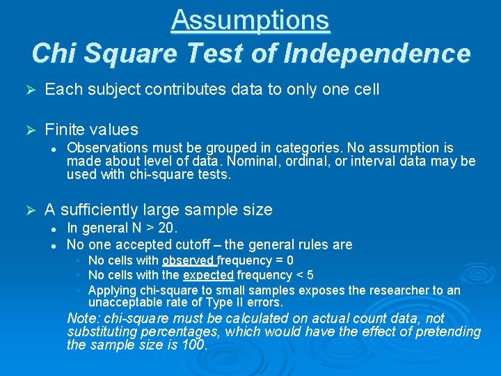
Assumptions Chi Square Test of Independence Ø Each subject contributes data to only one cell Ø Finite values l Ø Observations must be grouped in categories. No assumption is made about level of data. Nominal, ordinal, or interval data may be used with chi-square tests. A sufficiently large sample size l l In general N > 20. No one accepted cutoff – the general rules are • • • No cells with observed frequency = 0 No cells with the expected frequency < 5 Applying chi-square to small samples exposes the researcher to an unacceptable rate of Type II errors. Note: chi-square must be calculated on actual count data, not substituting percentages, which would have the effect of pretending the sample size is 100.

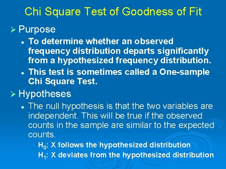
Chi Square Test of Goodness of Fit Ø Purpose l l To determine whether an observed frequency distribution departs significantly from a hypothesized frequency distribution. This test is sometimes called a One-sample Chi Square Test. Ø Hypotheses l The null hypothesis is that the two variables are independent. This will be true if the observed counts in the sample are similar to the expected counts. • • H 0: X follows the hypothesized distribution H 1: X deviates from the hypothesized distribution

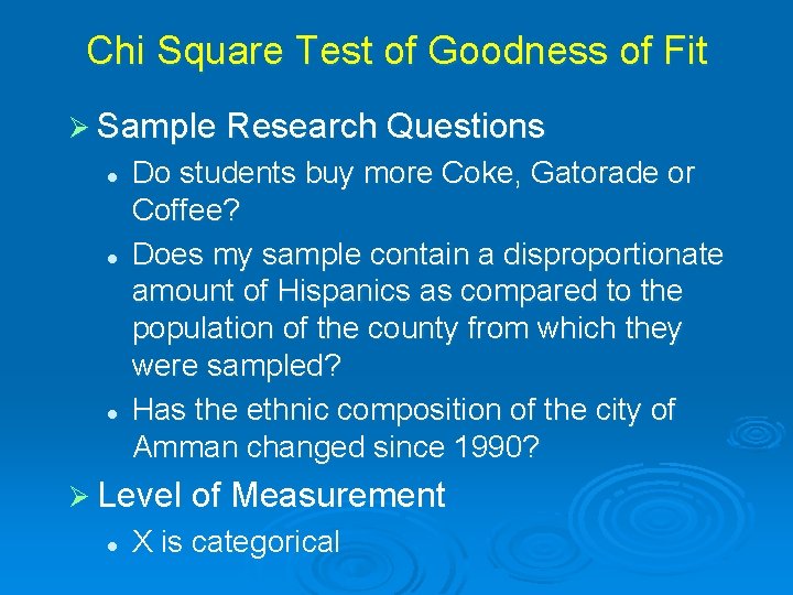
Chi Square Test of Goodness of Fit Ø Sample Research Questions l l l Do students buy more Coke, Gatorade or Coffee? Does my sample contain a disproportionate amount of Hispanics as compared to the population of the county from which they were sampled? Has the ethnic composition of the city of Amman changed since 1990? Ø Level of Measurement l X is categorical

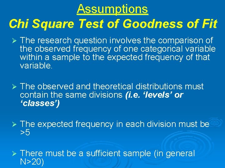
Assumptions Chi Square Test of Goodness of Fit Ø The research question involves the comparison of the observed frequency of one categorical variable within a sample to the expected frequency of that variable. Ø The observed and theoretical distributions must contain the same divisions (i. e. ‘levels’ or ‘classes’) Ø The expected frequency in each division must be >5 Ø There must be a sufficient sample (in general N>20)

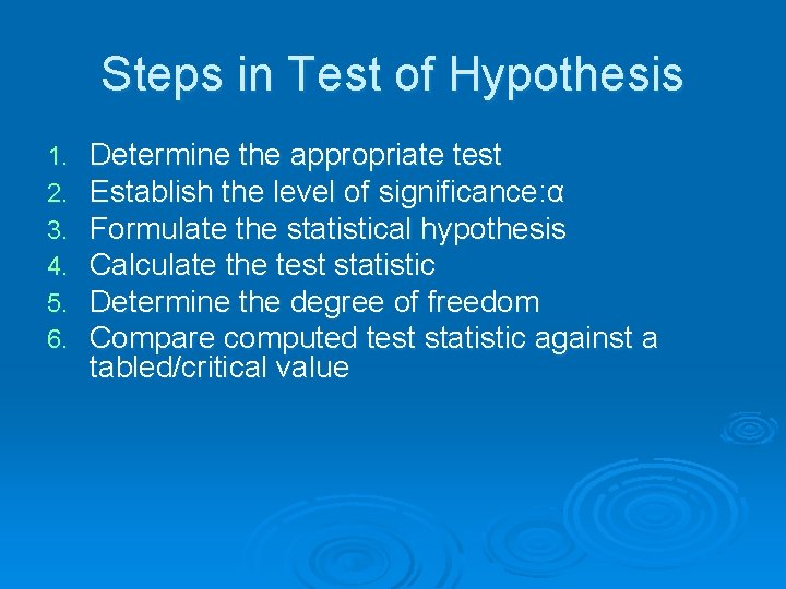
Steps in Test of Hypothesis 1. 2. 3. 4. 5. 6. Determine the appropriate test Establish the level of significance: α Formulate the statistical hypothesis Calculate the test statistic Determine the degree of freedom Compare computed test statistic against a tabled/critical value

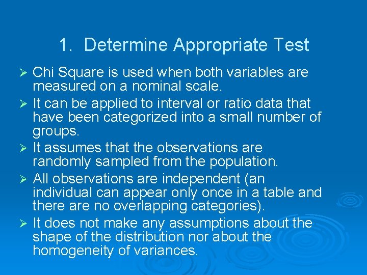
1. Determine Appropriate Test Chi Square is used when both variables are measured on a nominal scale. Ø It can be applied to interval or ratio data that have been categorized into a small number of groups. Ø It assumes that the observations are randomly sampled from the population. Ø All observations are independent (an individual can appear only once in a table and there are no overlapping categories). Ø It does not make any assumptions about the shape of the distribution nor about the homogeneity of variances. Ø

Establish Level of . 2 Significance Ø α is a predetermined value Ø The convention • • • α =. 05 α =. 01 α =. 001

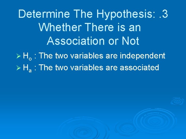
Determine The Hypothesis: . 3 Whether There is an Association or Not Ø Ho : The two variables are independent Ø Ha : The two variables are associated

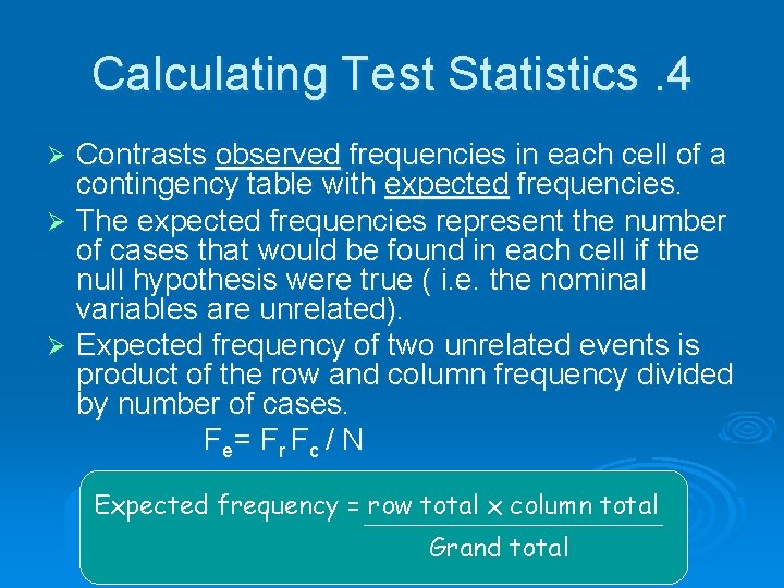
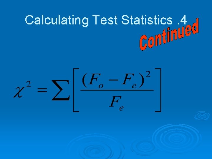
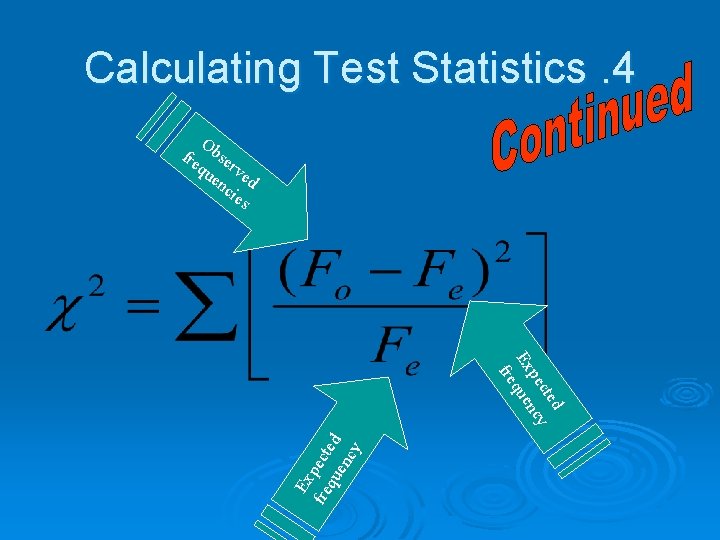
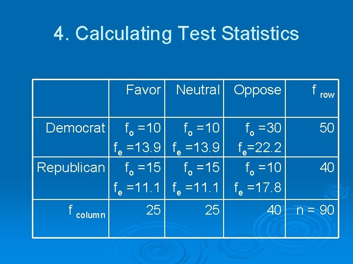
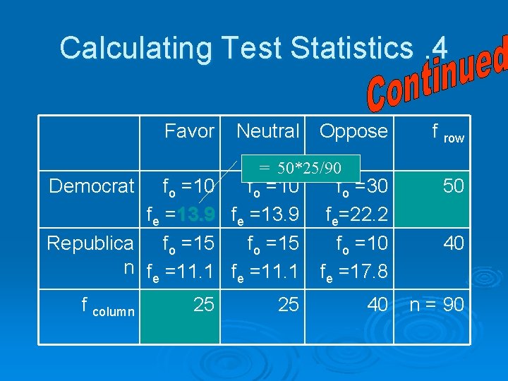
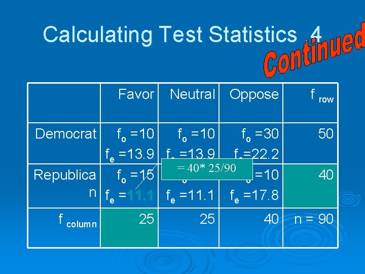
Calculating Test Statistics. 4 Contrasts observed frequencies in each cell of a contingency table with expected frequencies. Ø The expected frequencies represent the number of cases that would be found in each cell if the null hypothesis were true ( i. e. the nominal variables are unrelated). Ø Expected frequency of two unrelated events is product of the row and column frequency divided by number of cases. Fe= Fr Fc / N Ø Expected frequency = row total x column total Grand total

Calculating Test Statistics. 4

Calculating Test Statistics. 4 O fre bse qu rve en d cie s Ex fre pect qu ed en cy d cte pe ncy Ex que fre

Determine Degrees of . 5 Freedom df = (R-1)(C-1) f ber o Num ls in leve n m colu le ab vari Numbe r of leve ls i n r ow variabl e

6. Compare computed test statistic against a tabled/critical value Ø The computed value of the Pearson chi- square statistic is compared with the critical value to determine if the computed value is improbable Ø The critical tabled values are based on sampling distributions of the Pearson chi -square statistic Ø If calculated 2 is greater than 2 table value, reject Ho

Decision and Interpretation If the probability of the test statistic is less than or equal to the probability of the alpha error rate, we reject the null hypothesis and conclude that our data supports the research hypothesis. We conclude that there is a relationship between the variables. Ø If the probability of the test statistic is greater than the probability of the alpha error rate, we fail to reject the null hypothesis. We conclude that there is no relationship between the variables, i. e. they are independent. Ø

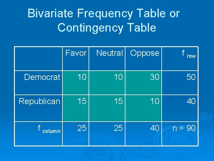
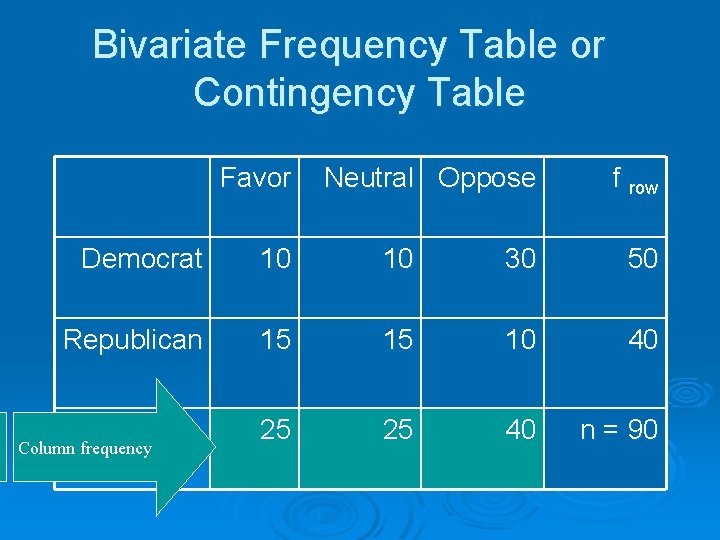
Example Ø Suppose a researcher is interested in voting preferences on gun control issues. Ø A questionnaire was developed and sent to a random sample of 90 voters. Ø The researcher also collects information about the political party membership of the sample of 90 respondents.

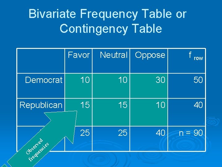
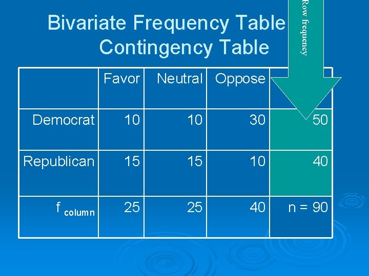
Bivariate Frequency Table or Contingency Table Favor Neutral Oppose f row Democrat 10 10 30 50 Republican 15 15 10 40 f column 25 25 40 n = 90

Bivariate Frequency Table or Contingency Table Favor Neutral Oppose f row Democrat 10 10 30 50 Republican 15 15 10 40 f column 25 25 40 n = 90 ed s v er cie s n Ob que fre

Row frequency Bivariate Frequency Table or Contingency Table Favor Neutral Oppose f row Democrat 10 10 30 50 Republican 15 15 10 40 f column 25 25 40 n = 90

Bivariate Frequency Table or Contingency Table Favor Neutral Oppose f row Democrat 10 10 30 50 Republican 15 15 10 40 f column Column frequency 25 25 40 n = 90

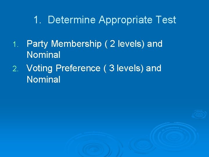
1. Determine Appropriate Test Party Membership ( 2 levels) and Nominal 2. Voting Preference ( 3 levels) and Nominal 1.

Establish Level of . 2 Significance Alpha of. 05

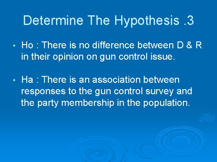
Determine The Hypothesis. 3 • Ho : There is no difference between D & R in their opinion on gun control issue. • Ha : There is an association between responses to the gun control survey and the party membership in the population.

4. Calculating Test Statistics Favor Neutral Oppose Democrat fo =10 fe =13. 9 Republican fo =15 fe =11. 1 f column 25 25 f row fo =30 fe=22. 2 fo =10 fe =17. 8 50 40 n = 90 40

Calculating Test Statistics. 4 Favor Neutral Oppose = 50*25/90 Democrat fo =10 fe =13. 9 Republica fo =15 n fe =11. 1 f column 25 25 f row fo =30 fe=22. 2 fo =10 fe =17. 8 50 40 n = 90 40

Calculating Test Statistics. 4 Favor Neutral Oppose f row fo =10 fo =30 fe =13. 9 fe=22. 2 = 40* 25/90 Republica fo =15 fo =10 n fe =11. 1 fe =17. 8 50 Democrat f column 25 25 40 40 n = 90

4. Calculating Test Statistics = 11. 03

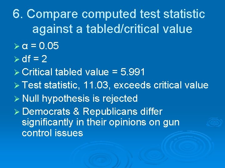
Determine Degrees of . 5 Freedom df = (R-1)(C-1) = (2 -1)(3 -1) = 2

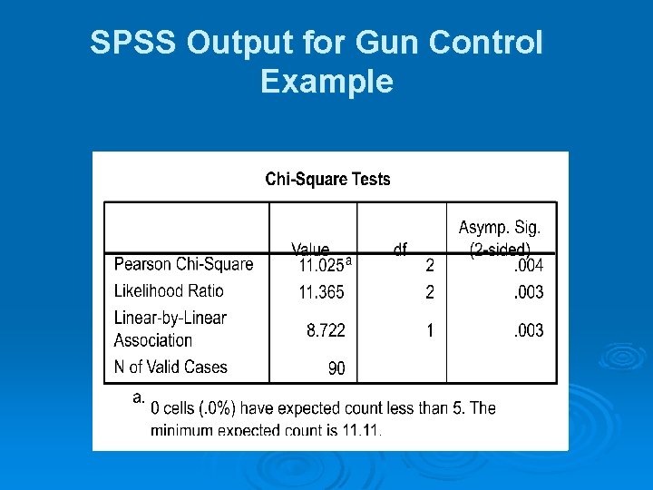
6. Compare computed test statistic against a tabled/critical value Ø α = 0. 05 Ø df = 2 Ø Critical tabled value = 5. 991 Ø Test statistic, 11. 03, exceeds critical value Ø Null hypothesis is rejected Ø Democrats & Republicans differ significantly in their opinions on gun control issues

SPSS Output for Gun Control Example

Additional Information in SPSS Output Ø Exceptions that might distort χ2 Assumptions l l Associations in some but not all categories Low expected frequency per cell Ø Extent of association is not same as statistical significance Demonstrated through an example

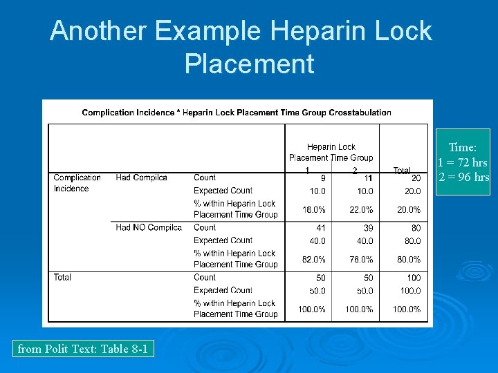
Another Example Heparin Lock Placement Time: 1 = 72 hrs 2 = 96 hrs from Polit Text: Table 8 -1

Hypotheses in Heparin Lock Placement Ø Ho: There is no association between complication incidence and length of heparin lock placement. (The variables are independent). Ø Ha: There is an association between complication incidence and length of heparin lock placement. (The variables are related).

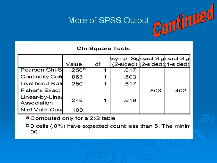
More of SPSS Output

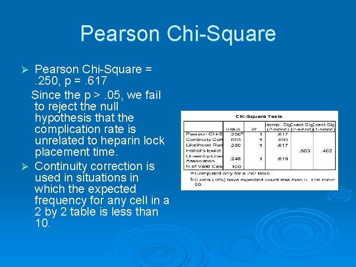
Pearson Chi-Square = . 250, p =. 617 Since the p >. 05, we fail to reject the null hypothesis that the complication rate is unrelated to heparin lock placement time. Ø Continuity correction is used in situations in which the expected frequency for any cell in a 2 by 2 table is less than 10. Ø

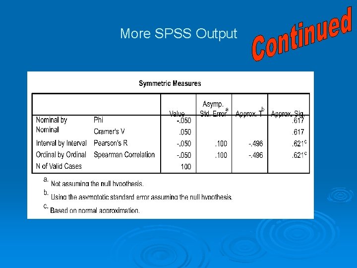
More SPSS Output

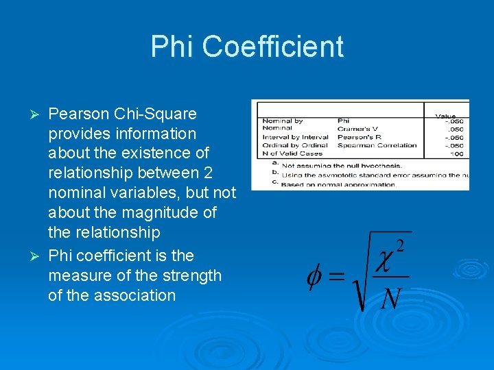
Phi Coefficient Pearson Chi-Square provides information about the existence of relationship between 2 nominal variables, but not about the magnitude of the relationship Ø Phi coefficient is the measure of the strength of the association Ø

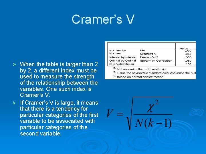
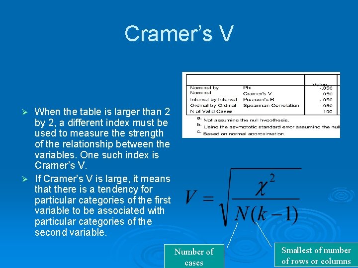
Cramer’s V When the table is larger than 2 by 2, a different index must be used to measure the strength of the relationship between the variables. One such index is Cramer’s V. Ø If Cramer’s V is large, it means that there is a tendency for particular categories of the first variable to be associated with particular categories of the second variable. Ø

Cramer’s V When the table is larger than 2 by 2, a different index must be used to measure the strength of the relationship between the variables. One such index is Cramer’s V. Ø If Cramer’s V is large, it means that there is a tendency for particular categories of the first variable to be associated with particular categories of the second variable. Ø Number of cases Smallest of number of rows or columns

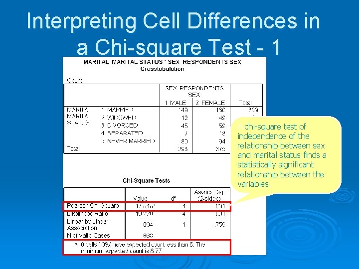
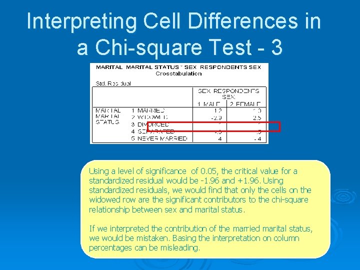
Interpreting Cell Differences in a Chi-square Test - 1 A chi-square test of independence of the relationship between sex and marital status finds a statistically significant relationship between the variables.

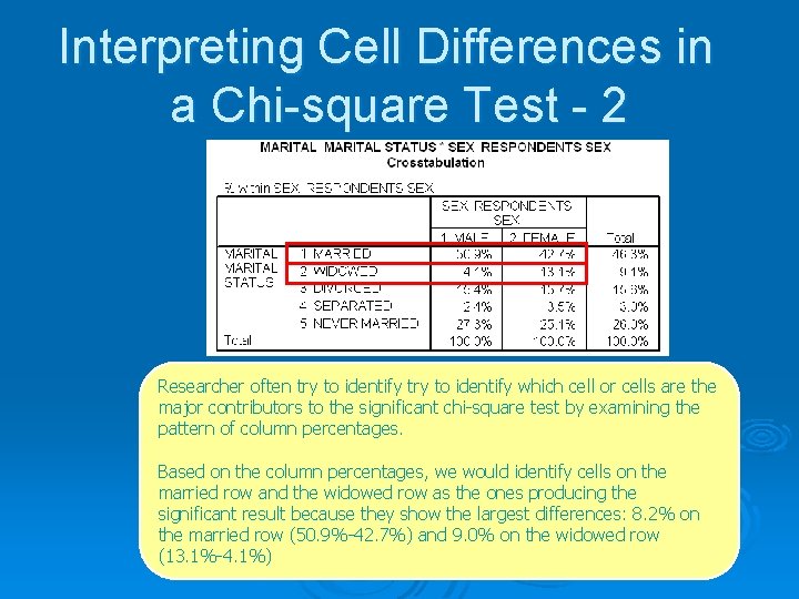
Interpreting Cell Differences in a Chi-square Test - 2 Researcher often try to identify which cell or cells are the major contributors to the significant chi-square test by examining the pattern of column percentages. Based on the column percentages, we would identify cells on the married row and the widowed row as the ones producing the significant result because they show the largest differences: 8. 2% on the married row (50. 9%-42. 7%) and 9. 0% on the widowed row (13. 1%-4. 1%)

Interpreting Cell Differences in a Chi-square Test - 3 Using a level of significance of 0. 05, the critical value for a standardized residual would be -1. 96 and +1. 96. Using standardized residuals, we would find that only the cells on the widowed row are the significant contributors to the chi-square relationship between sex and marital status. If we interpreted the contribution of the married marital status, we would be mistaken. Basing the interpretation on column percentages can be misleading.

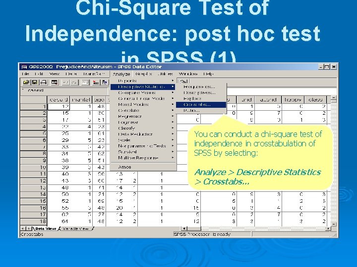
Chi-Square Test of Independence: post hoc test in SPSS (1) You can conduct a chi-square test of independence in crosstabulation of SPSS by selecting: Analyze > Descriptive Statistics > Crosstabs…

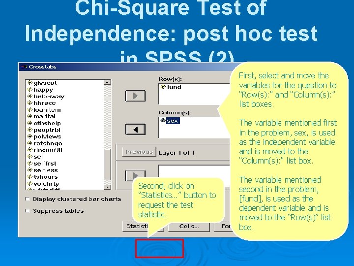
Chi-Square Test of Independence: post hoc test in SPSS (2) First, select and move the variables for the question to “Row(s): ” and “Column(s): ” list boxes. The variable mentioned first in the problem, sex, is used as the independent variable and is moved to the “Column(s): ” list box. Second, click on “Statistics…” button to request the test statistic. The variable mentioned second in the problem, [fund], is used as the dependent variable and is moved to the “Row(s)” list box.

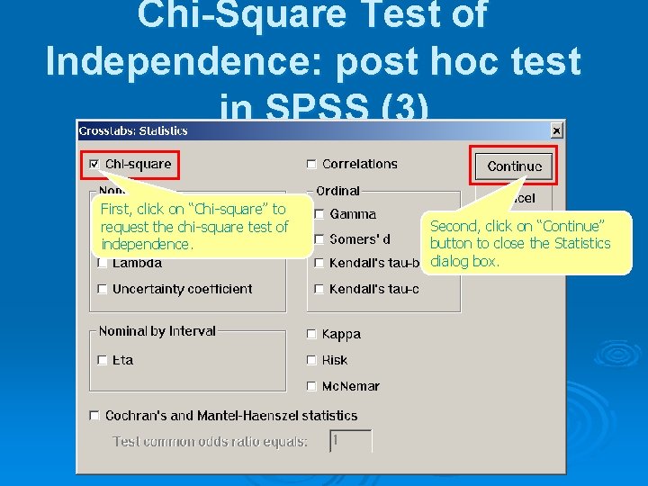
Chi-Square Test of Independence: post hoc test in SPSS (3) First, click on “Chi-square” to request the chi-square test of independence. Second, click on “Continue” button to close the Statistics dialog box.

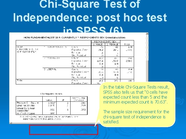
Chi-Square Test of Independence: post hoc test in SPSS (6) In the table Chi-Square Tests result, SPSS also tells us that “ 0 cells have expected count less than 5 and the minimum expected count is 70. 63”. The sample size requirement for the chi-square test of independence is satisfied.

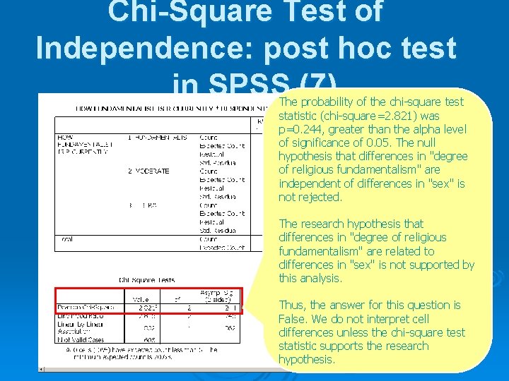
Chi-Square Test of Independence: post hoc test in SPSS (7) The probability of the chi-square test statistic (chi-square=2. 821) was p=0. 244, greater than the alpha level of significance of 0. 05. The null hypothesis that differences in "degree of religious fundamentalism" are independent of differences in "sex" is not rejected. The research hypothesis that differences in "degree of religious fundamentalism" are related to differences in "sex" is not supported by this analysis. Thus, the answer for this question is False. We do not interpret cell differences unless the chi-square test statistic supports the research hypothesis.

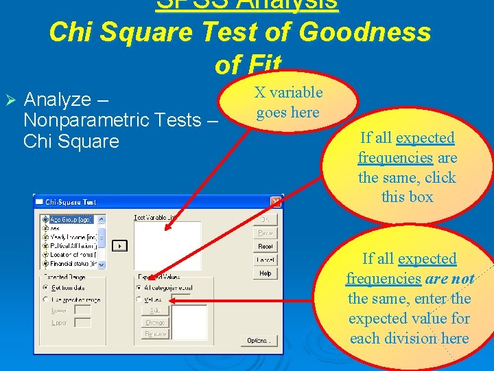
SPSS Analysis Chi Square Test of Goodness of Fit Ø Analyze – Nonparametric Tests – Chi Square X variable goes here If all expected frequencies are the same, click this box If all expected frequencies are not the same, enter the expected value for each division here

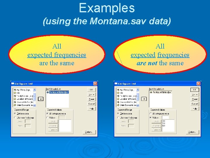
Examples (using the Montana. sav data) All expected frequencies are the same All expected frequencies are not the same

Thank You for Listening Questions?