Ted Adelsons checkerboard illusion Motion illusion rotating snakes

Ted Adelson’s checkerboard illusion

Motion illusion, rotating snakes

Sampling and Reconstruction 2 Slides from Alexei Efros, Fei Li, Steve Marschner, and others CS 195 g: Computational Photography James Hays, Brown, Spring 2010

Detailed Recap of Wednesday

Slide credit Fei Li

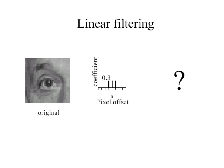
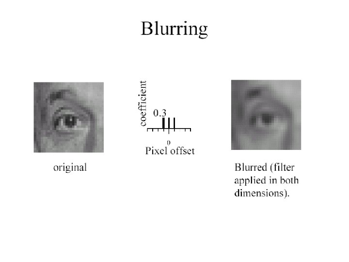
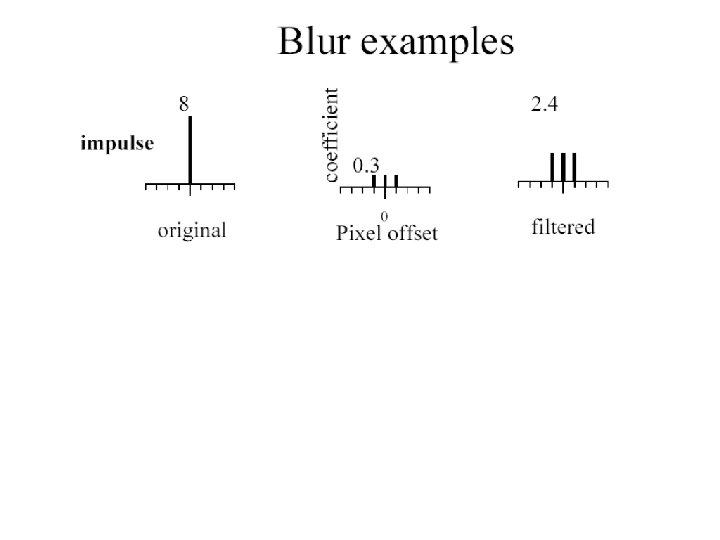
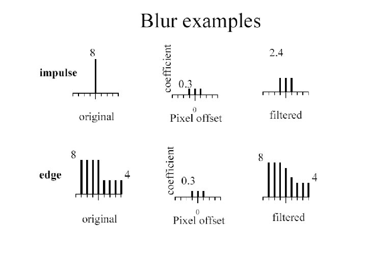
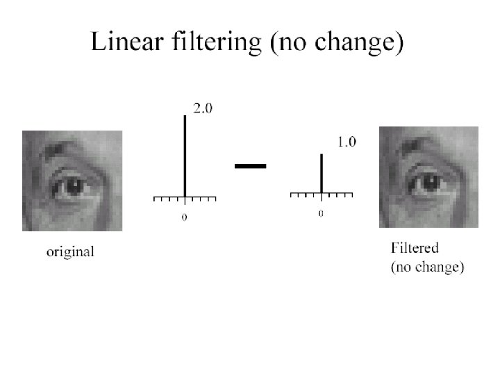
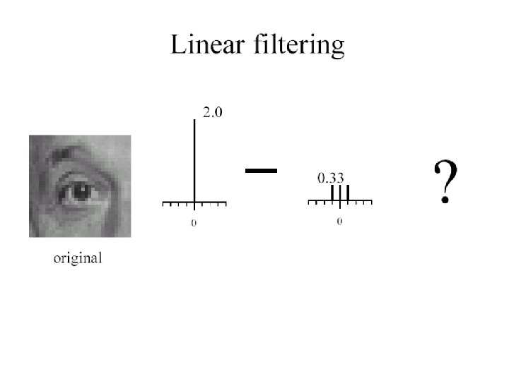
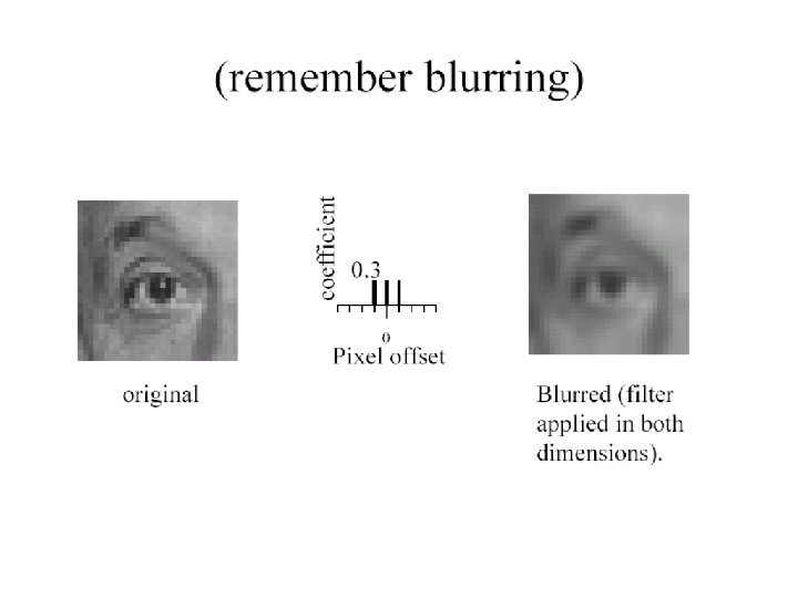
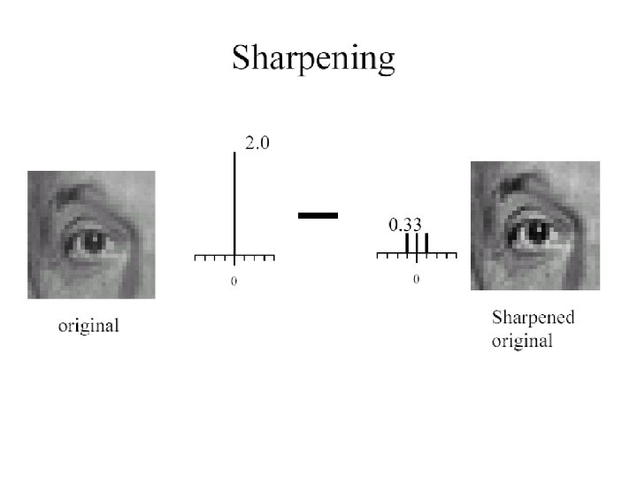
Image half-sizing This image is too big to fit on the screen. How can we reduce it? How to generate a halfsized version?

Image sub-sampling 1/8 1/4 Throw away every other row and column to create a 1/2 size image - called image sub-sampling Slide by Steve Seitz

Image sub-sampling 1/2 1/4 (2 x zoom) 1/8 (4 x zoom) Aliasing! What do we do? Slide by Steve Seitz

Gaussian (lowpass) pre-filtering G 1/8 G 1/4 Gaussian 1/2 Solution: filter the image, then subsample • Filter size should double for each ½ size reduction. Why? Slide by Steve Seitz

Subsampling with Gaussian pre-filtering Gaussian 1/2 G 1/4 G 1/8 Slide by Steve Seitz

Compare with. . . 1/2 1/4 (2 x zoom) 1/8 (4 x zoom) Slide by Steve Seitz

Gaussian (lowpass) pre-filtering G 1/8 G 1/4 Gaussian 1/2 Solution: filter the image, then subsample • Filter size should double for each ½ size reduction. Why? Slide by Steve Seitz • How can we speed this up?

Image Pyramids Known as a Gaussian Pyramid [Burt and Adelson, 1983] • In computer graphics, a mip map [Williams, 1983] • A precursor to wavelet transform Slide by Steve Seitz

A bar in the big images is a hair on the zebra’s nose; in smaller images, a stripe; in the smallest, the animal’s nose Figure from David Forsyth

What are they good for? Improve Search • Search over translations – Like project 1 – Classic coarse-to-fine strategy • Search over scale – Template matching – E. g. find a face at different scales Pre-computation • Need to access image at different blur levels • Useful for texture mapping at different resolutions (called mip -mapping)

Gaussian pyramid construction filter mask Repeat • Filter • Subsample Until minimum resolution reached • can specify desired number of levels (e. g. , 3 -level pyramid) The whole pyramid is only 4/3 the size of the original image! Slide by Steve Seitz

Continuous convolution: warm-up • Can apply sliding-window average to a continuous function just as

Continuous convolution • Sliding average expressed mathematically: – note difference in normalization (only for box) • Convolution just adds weights – weighting is now by a function – weighted integral is like weighted average – again bounds are set by support of f(x) © 2006 Steve Marschner • 46

One more convolution • Continuous–discrete convolution – used for reconstruction and resampling © 2006

Reconstruction © 2006 Steve Marschner • 48

Resampling • Changing the sample rate – in images, this is enlarging and reducing • Creating more samples: – increasing the sample rate – “upsampling” – “enlarging” • Ending up with fewer samples: – decreasing the sample rate – “downsampling” – “reducing” © 2006 Steve Marschner • 49

Resampling • Reconstruction creates a continuous function – forget its origins, go ahead and

Cont. –disc. convolution in 2 D • same convolution—just two variables now – loop over nearby pixels, average using filter weight – looks like discrete filter, but offsets are not integers and filter is continuous – remember placement of filter relative to grid is variable © 2006 Steve Marschner • 51

A gallery of filters • Box filter – Simple and cheap • Tent filter

Effects of reconstruction filters • For some filters, the reconstruction process winds up implementing a simple algorithm • Box filter (radius 0. 5): nearest neighbor sampling – box always catches exactly one input point – it is the input point nearest the output point – so output[i, j] = input[round(x(i)), round(y(j))] x(i) computes the position of the output coordinate i on the input grid • Tent filter (radius 1): linear interpolation – tent catches exactly 2 input points – weights are a and (1 – a) – result is straight-line interpolation from one point to the next © 2006 Steve Marschner • 57

Properties of filters • Degree of continuity • Impulse response • Interpolating or no

Ringing, overshoot, ripples • Overshoot – caused by negative filter values • Ripples –

Yucky details • What about near the edge? – the filter window falls off the edge of the image – need to extrapolate – methods: • • • clip filter (black) wrap around copy edge reflect across edge vary filter near edge © 2006 Steve Marschner • 60

Median filters • A Median Filter operates over a window by selecting the median intensity in the window. • What advantage does a median filter have over a mean filter? • Is a median filter a kind of convolution? Slide by Steve Seitz © 2006 Steve Marschner • 61