Skeletons for Parallel Scientific Computing David Duke Computational

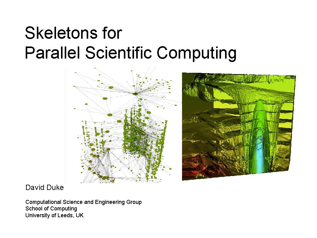
Skeletons for Parallel Scientific Computing David Duke Computational Science and Engineering Group School of Computing University of Leeds, UK

The purpose of computing is insight, not numbers. R. Hamming, Numerical Methods for Scientists and Engineers, 1962.

Outline 1. Background • • • Computational science & visualization Topological analysis Running case study: the Joint Contour Net (JCN) and its implementation 2. Sequential implementation 3. Skeletons 4. Shared-memory parallelism in the Par Monad 5. Distributed parallelism • • Eden Distributed skeletons Performance Distributed data representation 6. Insight and conclusions • • Strengths and weaknesses of skeletons Challenges and opportunities in functional HPC

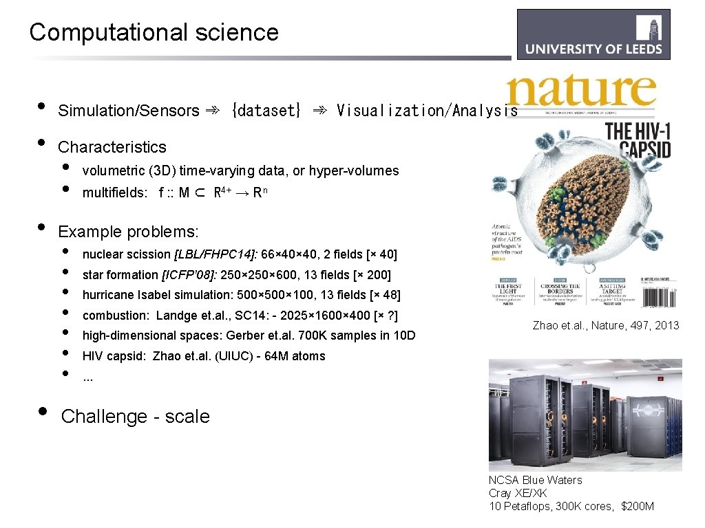
Computational science • • Simulation/Sensors ➾ {dataset} ➾ Visualization/Analysis Characteristics • • volumetric (3 D) time-varying data, or hyper-volumes multifields: f : : M ⊂ R 4+ → Rn Example problems: • • nuclear scission [LBL/FHPC 14]: 66× 40, 2 fields [× 40] star formation [ICFP’ 08]: 250× 600, 13 fields [× 200] hurricane Isabel simulation: 500× 100, 13 fields [× 48] combustion: Landge et. al. , SC 14: - 2025× 1600× 400 [× ? ] high-dimensional spaces: Gerber et. al. 700 K samples in 10 D Zhao et. al. , Nature, 497, 2013 HIV capsid: Zhao et. al. (UIUC) - 64 M atoms. . . Challenge - scale NCSA Blue Waters Cray XE/XK 10 Petaflops, 300 K cores, $200 M

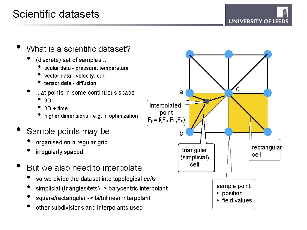
Scientific datasets • What is a scientific dataset? • • (discrete) set of samples. . . • • • scalar data - pressure, temperature vector data - velocity, curl tensor data - diffusion a . . at points in some continuous space • • • 3 D 3 D + time higher dimensions - e. g. in optimization interpolated point Fp= f(Fa, Fb, Fc) Sample points may be • • b organised on a regular grid irregularly spaced But we also need to interpolate • • c rectangular cell triangular (simplicial) cell so we divide the dataset into topological cells simplicial (triangles/tets) -> barycentric interpolant square/rectangular -> bi/trilinear interpolant other subdivisions and interpolants used sample point • position • field values

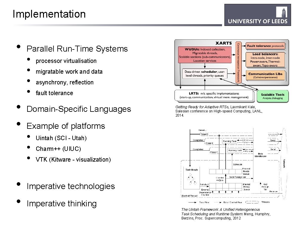
Implementation • • • Parallel Run-Time Systems • • processor virtualisation migratable work and data asynchrony, reflection fault tolerance Domain-Specific Languages Getting Ready for Adaptive RTSs, Laxmikant Kale, Salesian conference on High-speed Computing, LANL, 2014. Example of platforms • • • Uintah (SCI - Utah) Charm++ (UIUC) VTK (Kitware - visualization) Imperative technologies Imperative thinking The Uintah Framework: A Unified Heterogeneous Task Scheduling and Runtime System: Meng, Humphry, Berzins, Proc. Supercomputing, 2012

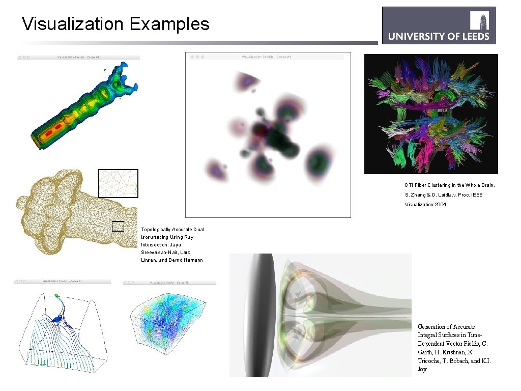
Visualization Examples DTI Fiber Clustering in the Whole Brain, S. Zhang & D. Laidlaw, Proc. IEEE Visualization 2004. Topologically Accurate Dual Isosurfacing Using Ray Intersection: Jaya Sreevalsan-Nair, Lars Linsen, and Bernd Hamann Generation of Accurate Integral Surfaces in Time. Dependent Vector Fields, C. Garth, H. Krishnan, X. Tricoche, T. Bobach, and K. I. Joy

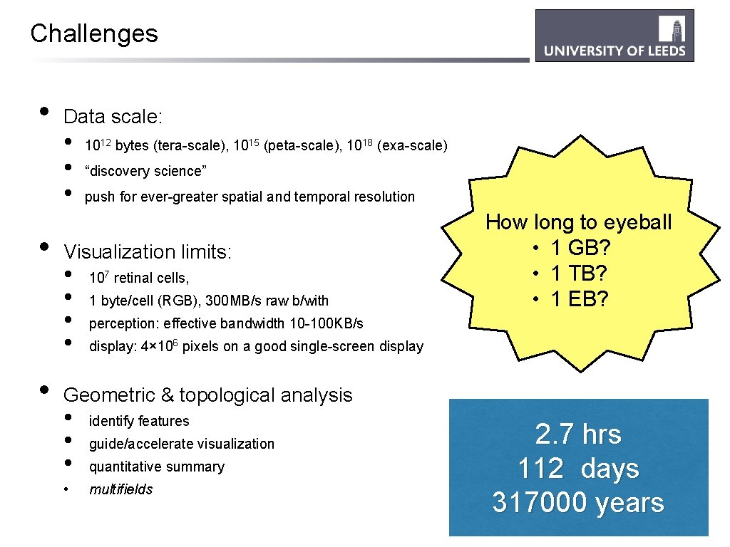
Challenges • • • Data scale: • • • 1012 bytes (tera-scale), 1015 (peta-scale), 1018 (exa-scale) “discovery science” push for ever-greater spatial and temporal resolution Visualization limits: • • 107 retinal cells, 1 byte/cell (RGB), 300 MB/s raw b/with How long to eyeball • 1 GB? • 1 TB? • 1 EB? perception: effective bandwidth 10 -100 KB/s display: 4× 106 pixels on a good single-screen display Geometric & topological analysis • • identify features guide/accelerate visualization quantitative summary multifields 2. 7 hrs 112 days 317000 years

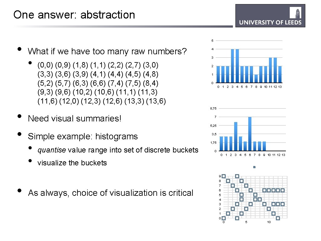
One answer: abstraction • • 5 What if we have too many raw numbers? • (0, 0) (0, 9) (1, 8) (1, 1) (2, 2) (2, 7) (3, 0) (3, 3) (3, 6) (3, 9) (4, 1) (4, 4) (4, 5) (4, 8) (5, 2) (5, 7) (6, 3) (6, 6) (7, 4) (7, 5) (8, 4) (9, 3) (9, 6) (10, 2) (10, 6) (11, 1) (11, 3) (11, 6) (12, 0) (12, 3) (12, 6) (13, 3) (13, 6) 4 3 2 1 0 0 1 2 3 4 5 6 7 8 9 10 11 12 13 8, 75 Need visual summaries! 7 5, 25 Simple example: histograms • • quantise value range into set of discrete buckets 3, 5 1, 75 0 0 1 2 3 4 5 6 7 8 9 10 11 12 13 visualize the buckets As always, choice of visualization is critical 9 8 7 6 5 4 3 2 1 0 0 5 10

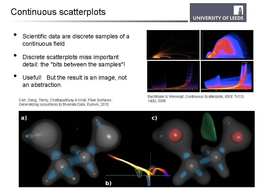
Continuous scatterplots • • • Scientific data are discrete samples of a continuous field Discrete scatterplots miss important detail: the "bits between the samples"! Useful! But the result is an image, not an abstraction. Carr, Geng, Tierny, Chattopadhyay & Knoll, Fiber Surfaces: Generalizing Isosurfaces to Bivariate Data, Eurovis, 2015. Bachthaler & Weiskopf, Continuous Scatterplots, IEEE TVCG 14(6), 2008

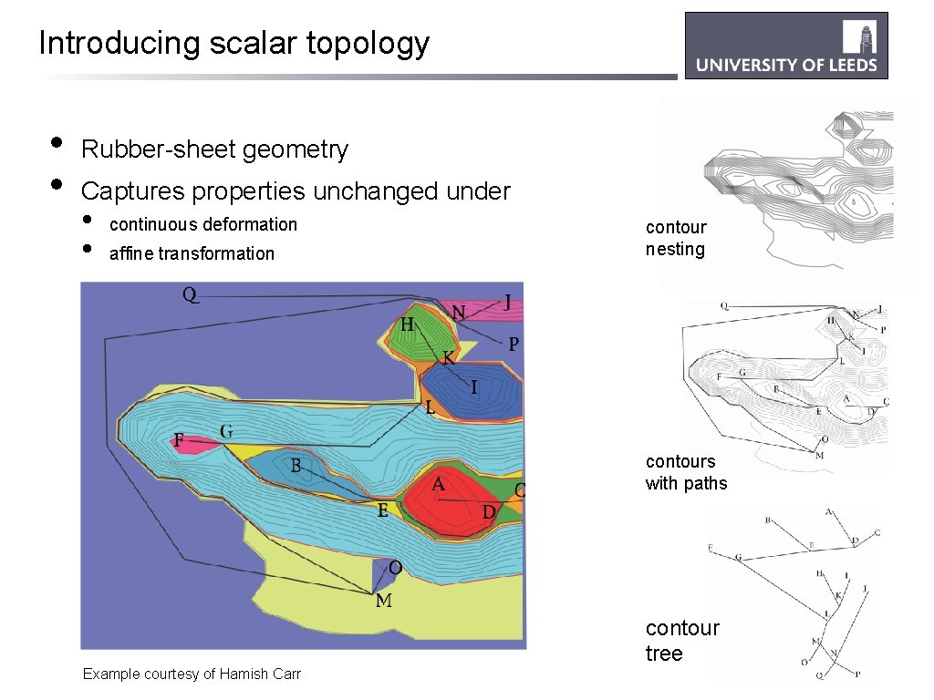
Introducing scalar topology • • Rubber-sheet geometry Captures properties unchanged under • • continuous deformation affine transformation contour nesting contours with paths contour tree Example courtesy of Hamish Carr

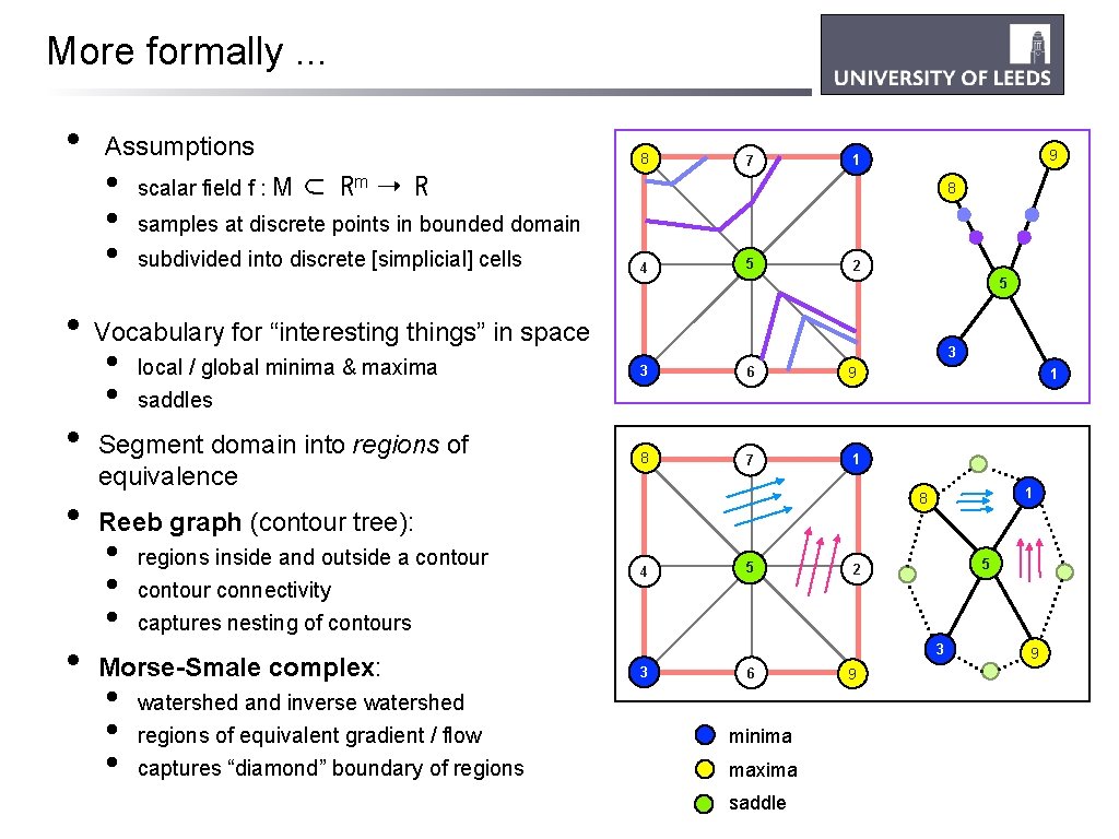
More formally. . . • Assumptions • • • scalar field f : M 8 7 9 1 ⊂ Rm ➝ R 8 samples at discrete points in bounded domain subdivided into discrete [simplicial] cells 4 5 2 5 • Vocabulary for “interesting things” in space • • • local / global minima & maxima saddles Segment domain into regions of equivalence 3 3 6 9 8 7 1 1 1 8 Reeb graph (contour tree): • • • regions inside and outside a contour connectivity captures nesting of contours Morse-Smale complex: • • • watershed and inverse watershed regions of equivalent gradient / flow captures “diamond” boundary of regions 4 5 5 2 3 3 6 minima maxima saddle 9 9

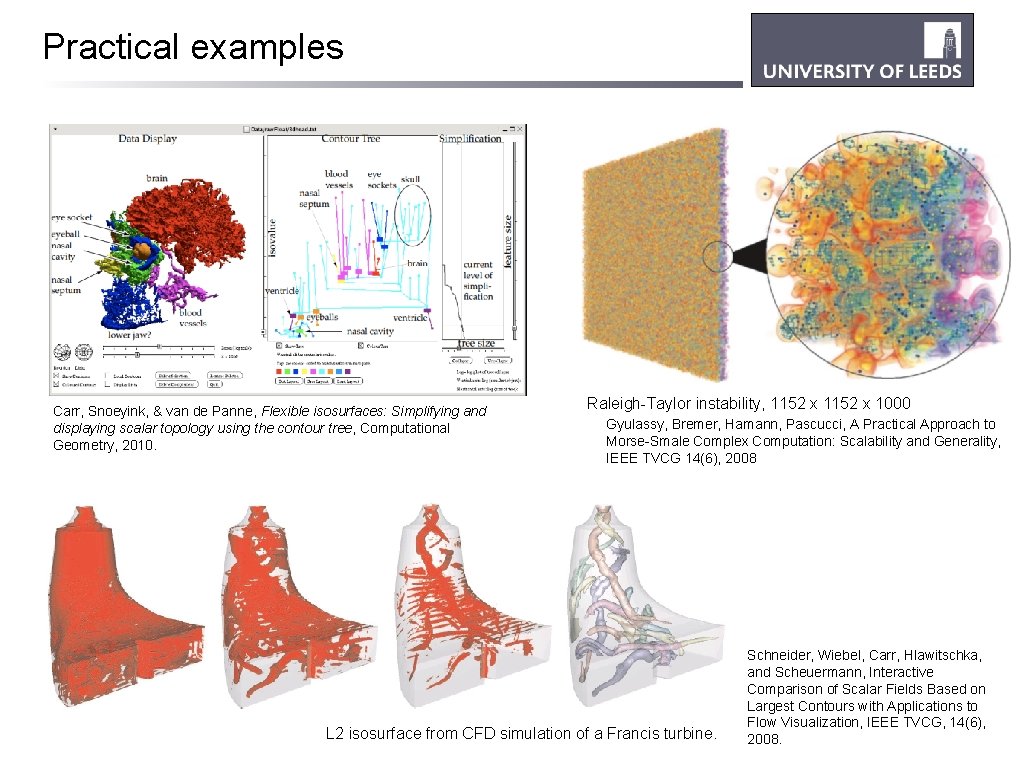
Practical examples Carr, Snoeyink, & van de Panne, Flexible isosurfaces: Simplifying and displaying scalar topology using the contour tree, Computational Geometry, 2010. Raleigh-Taylor instability, 1152 x 1000 Gyulassy, Bremer, Hamann, Pascucci, A Practical Approach to Morse-Smale Complex Computation: Scalability and Generality, IEEE TVCG 14(6), 2008 L 2 isosurface from CFD simulation of a Francis turbine. Schneider, Wiebel, Carr, Hlawitschka, and Scheuermann, Interactive Comparison of Scalar Fields Based on Largest Contours with Applications to Flow Visualization, IEEE TVCG, 14(6), 2008.

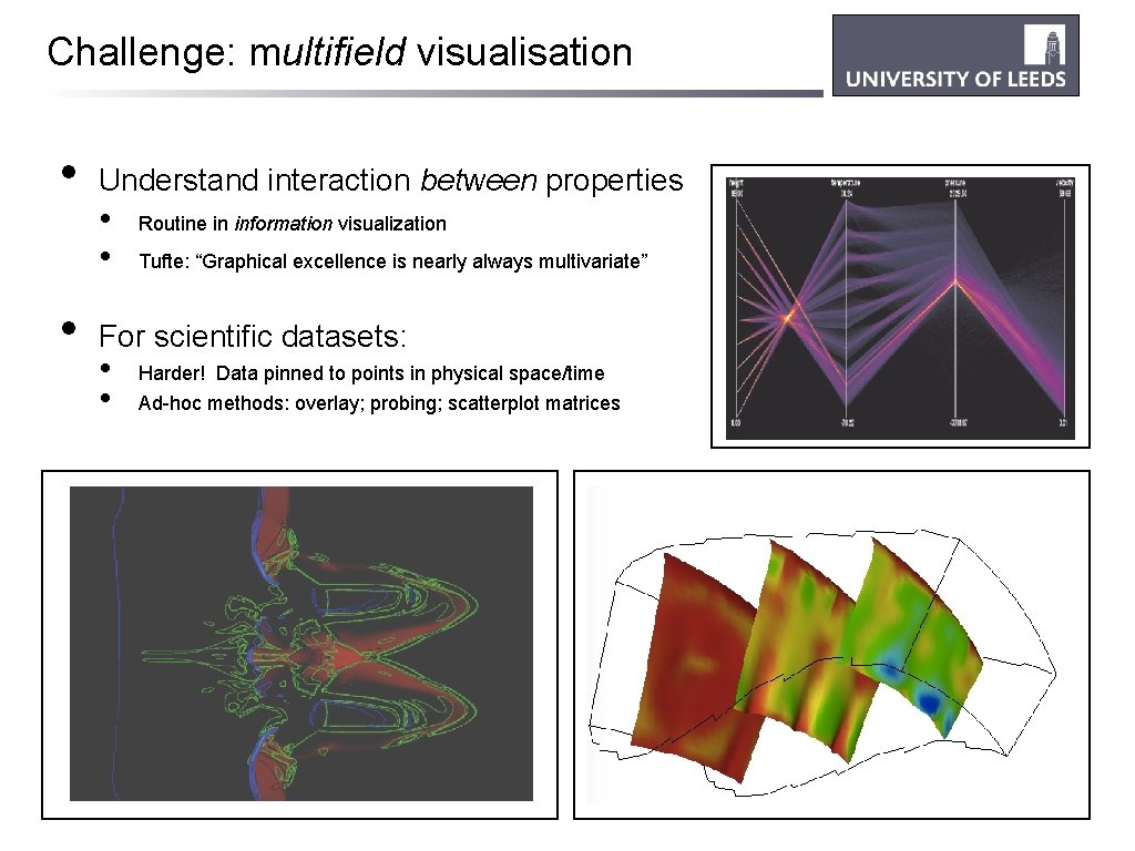
Challenge: multifield visualisation • • Understand interaction between properties • • Routine in information visualization Tufte: “Graphical excellence is nearly always multivariate” For scientific datasets: • • Harder! Data pinned to points in physical space/time Ad-hoc methods: overlay; probing; scatterplot matrices

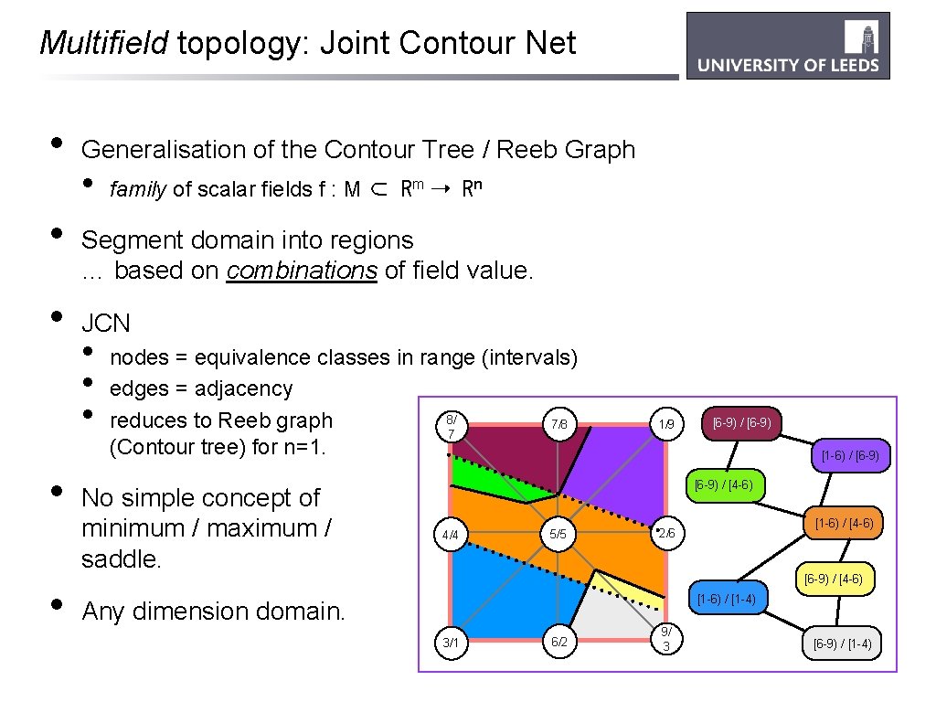
Multifield topology: Joint Contour Net • • • Generalisation of the Contour Tree / Reeb Graph • family of scalar fields f : M ⊂ Rm ➝ Rn Segment domain into regions … based on combinations of field value. JCN • • • nodes = equivalence classes in range (intervals) edges = adjacency 8/ reduces to Reeb graph 7/8 7 (Contour tree) for n=1. No simple concept of minimum / maximum / saddle. 1/9 [6 -9) / [6 -9) [1 -6) / [6 -9) / [4 -6) 4/4 5/5 [1 -6) / [4 -6) 2/6 [6 -9) / [4 -6) [1 -6) / [1 -4) Any dimension domain. 3/1 6/2 9/ 3 [6 -9) / [1 -4)

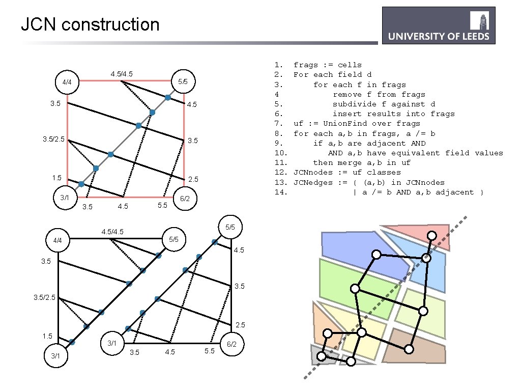
JCN construction 1. 2. 3. 4 5. 6. 7. 8. 9. 10. 11. 12. 13. 14. 4. 5/4. 5 5/5 4/4 3. 5 4. 5 3. 5/2. 5 3. 5 1. 5 2. 5 3/1 4. 5 3. 5 6/2 5. 5 5/5 4. 5/4. 5 5/5 4/4 4. 5 3. 5/2. 5 1. 5 3/1 3. 5 4. 5 5. 5 6/2 frags : = cells For each field d for each f in frags remove f from frags subdivide f against d insert results into frags uf : = Union. Find over frags for each a, b in frags, a /= b if a, b are adjacent AND a, b have equivalent field values then merge a, b in uf JCNnodes : = uf classes JCNedges : = { (a, b) in JCNnodes | a /= b AND a, b adjacent }

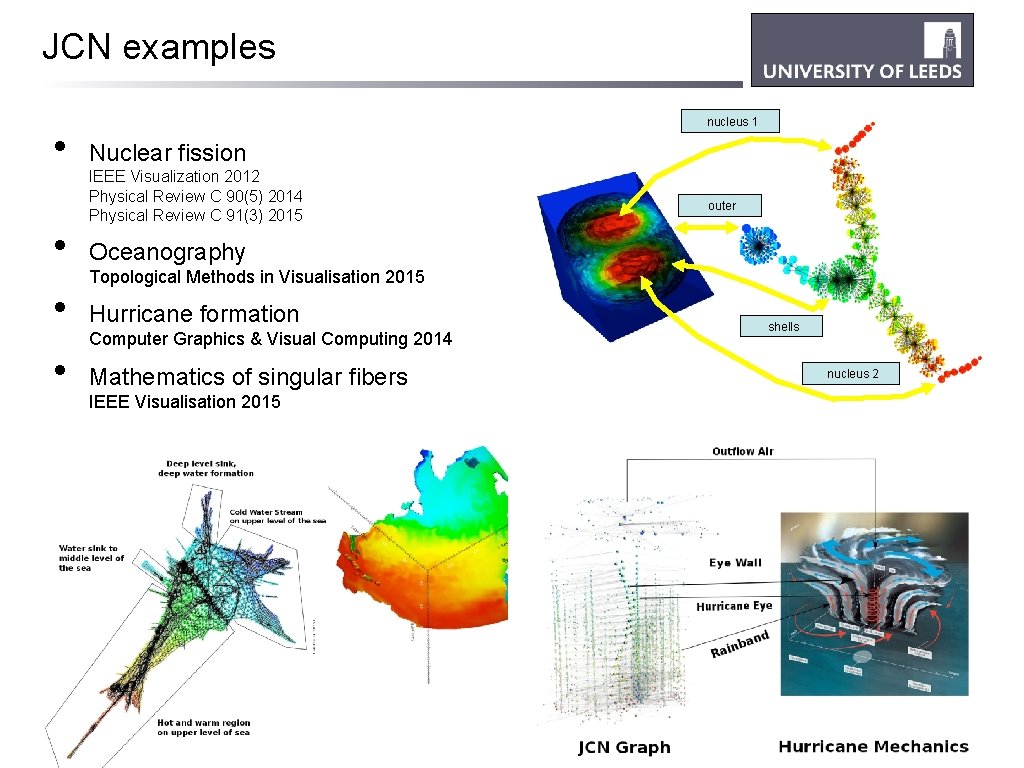
JCN examples • • nucleus 1 Nuclear fission IEEE Visualization 2012 Physical Review C 90(5) 2014 Physical Review C 91(3) 2015 outer Oceanography Topological Methods in Visualisation 2015 Hurricane formation Computer Graphics & Visual Computing 2014 Mathematics of singular fibers IEEE Visualisation 2015 shells nucleus 2

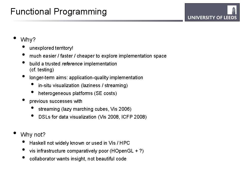
Functional Programming • Why? • • • unexplored territory! much easier / faster / cheaper to explore implementation space build a trusted reference implementation (cf. testing) longer-term aims: application-quality implementation • • in-situ visualization (laziness / streaming) heterogeneous platforms (SE costs) previous successes with • • streaming (lazy marching cubes, Vis 2006) DSLs for data visualization (Vis 2008, ICFP 2008) Why not? • • • Haskell not widely known or used in Vis / HPC vis infrastructure comparatively poor (HOpen. GL + ? ) collaborator wants insight, not beautiful code

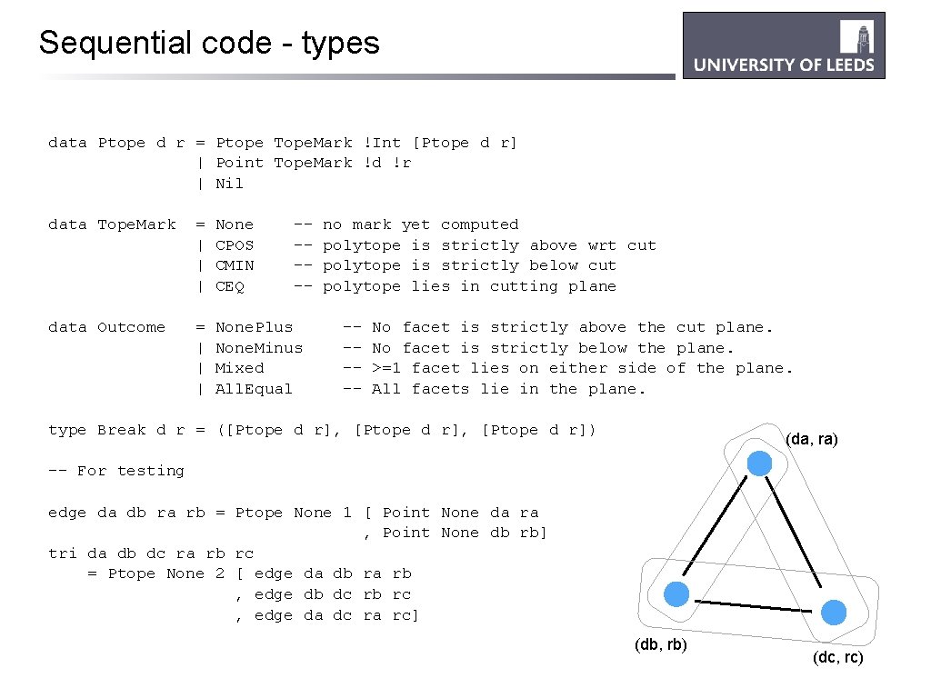
Sequential code - types data Ptope d r = Ptope Tope. Mark !Int [Ptope d r] | Point Tope. Mark !d !r | Nil data Tope. Mark = | | | None CPOS CMIN CEQ ----- data Outcome = | | | None. Plus None. Minus Mixed All. Equal no mark yet computed polytope is strictly above wrt cut polytope is strictly below cut polytope lies in cutting plane ----- No facet is strictly above the cut plane. No facet is strictly below the plane. >=1 facet lies on either side of the plane. All facets lie in the plane. type Break d r = ([Ptope d r], [Ptope d r]) (da, ra) -- For testing edge da db ra rb = Ptope None 1 [ Point None da ra , Point None db rb] tri da db dc ra rb rc = Ptope None 2 [ edge da db ra rb , edge db dc rb rc , edge da dc ra rc] (db, rb) (dc, rc)

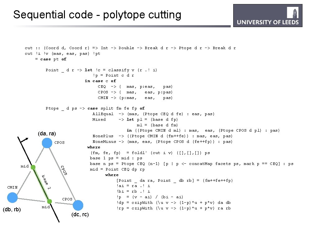
Sequential code - polytope cutting cut : : (Coord d, Coord r) => Int -> Double -> Break d r -> Ptope d r -> Break d r cut !i !v (mas, eas, pas) !pt = case pt of Point _ d r -> let !c = classify v (r. ! i) !p = Point c d r in case c of CEQ -> ( mas, p: eas, pas) CPOS -> ( mas, eas, p: pas) CMIN -> (p: mas, eas, pas) OS CP mid Ptope _ d ps -> case split fm fe fp of All. Equal -> (mas, (Ptope CEQ d fe) : eas, pas) Mixed -> let pl = (base d fp) ml = (base d fm) in ((Ptope CMIN d ml) : mas, eas, (Ptope CPOS d pl) : pas) (da, ra) None. Plus -> ((Ptope CMIN d (fm++fe)) : mas, eas, pas) None. Minus -> (mas, eas, (Ptope CPOS d (fe++fp)) : pas) CPOS where (fm, fe, fp) = foldl' (cut i v) ([], []) ps base 1 ps = mid : ps base n ps = Ptope CEQ (n-1) [p | p <- concat. Map facets ps, mark p == CEQ] : ps mid = Point CEQ dp rp where [Point _ da ra, Point _ db rb] = (fm++fe++fp) !ai = ra. ! i !bi = rb. ! i !p = (v - ai) / (bi - ai) CPOS !dp = czip. With (u v -> (1 -p)*u + p*v) da db mid !rp = czip. With (u v -> (1 -p)*u + p*v) ra rb 2 (db, rb) e s ba CMIN (dc, rc)

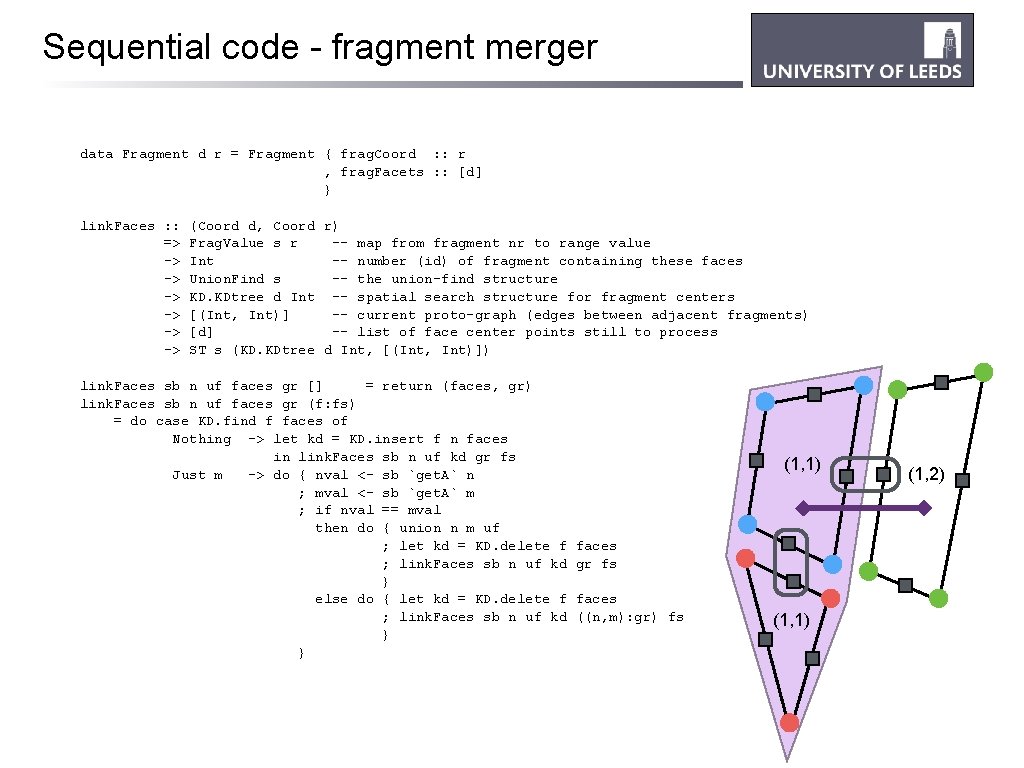
Sequential code - fragment merger data Fragment d r = Fragment { frag. Coord : : r , frag. Facets : : [d] } link. Faces : : => -> -> -> (Coord d, Coord r) Frag. Value s r -- map from fragment nr to range value Int -- number (id) of fragment containing these faces Union. Find s -- the union-find structure KD. KDtree d Int -- spatial search structure for fragment centers [(Int, Int)] -- current proto-graph (edges between adjacent fragments) [d] -- list of face center points still to process ST s (KD. KDtree d Int, [(Int, Int)]) link. Faces sb n uf faces gr [] = return (faces, gr) link. Faces sb n uf faces gr (f: fs) = do case KD. find f faces of Nothing -> let kd = KD. insert f n faces in link. Faces sb n uf kd gr fs Just m -> do { nval <- sb `get. A` n ; mval <- sb `get. A` m ; if nval == mval then do { union n m uf ; let kd = KD. delete f ; link. Faces sb n uf kd } else do { let kd = KD. delete f ; link. Faces sb n uf kd } } (1, 1) faces gr fs faces ((n, m): gr) fs (1, 1) (1, 2)

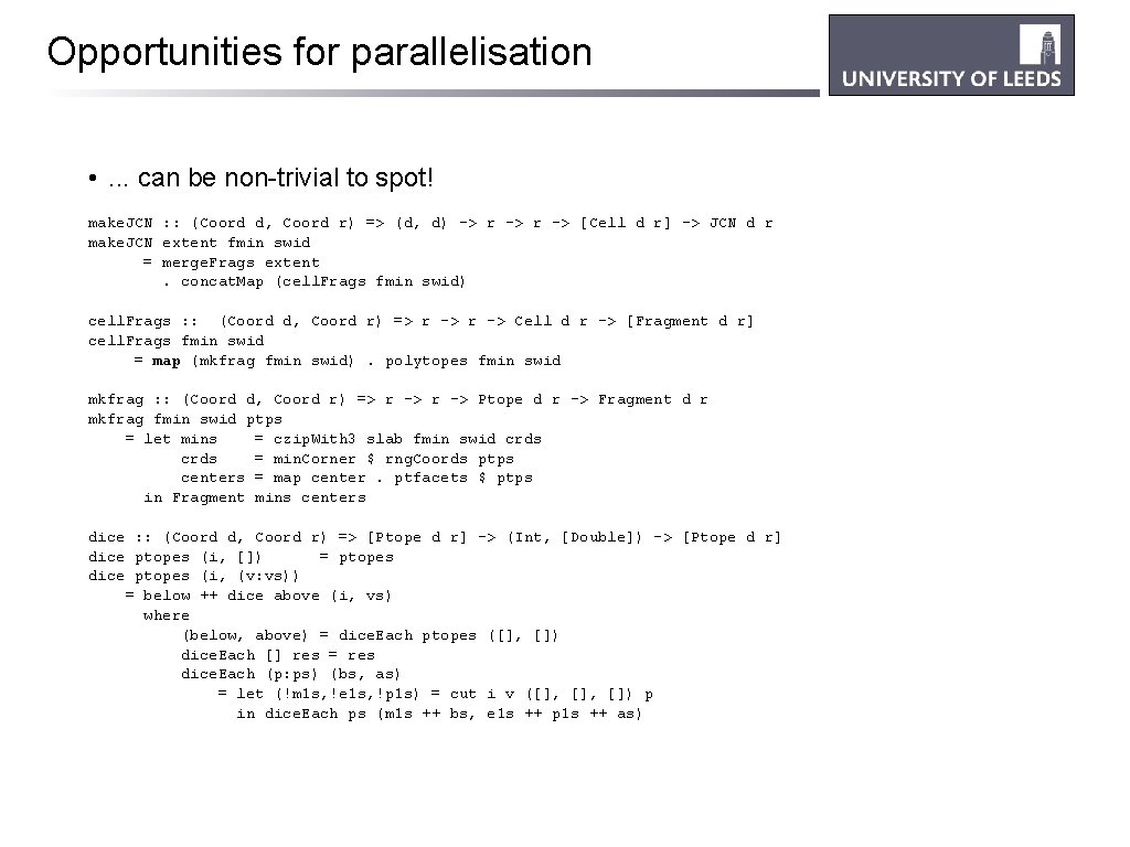
Opportunities for parallelisation • . . . can be non-trivial to spot! make. JCN : : (Coord d, Coord r) => (d, d) -> r -> [Cell d r] -> JCN d r make. JCN extent fmin swid = merge. Frags extent. concat. Map (cell. Frags fmin swid) cell. Frags : : (Coord d, Coord r) => r -> Cell d r -> [Fragment d r] cell. Frags fmin swid = map (mkfrag fmin swid). polytopes fmin swid mkfrag : : (Coord d, Coord r) => r -> Ptope d r -> Fragment d r mkfrag fmin swid ptps = let mins = czip. With 3 slab fmin swid crds = min. Corner $ rng. Coords ptps centers = map center. ptfacets $ ptps in Fragment mins centers dice : : (Coord d, Coord r) => [Ptope d r] -> (Int, [Double]) -> [Ptope d r] dice ptopes (i, []) = ptopes dice ptopes (i, (v: vs)) = below ++ dice above (i, vs) where (below, above) = dice. Each ptopes ([], []) dice. Each [] res = res dice. Each (p: ps) (bs, as) = let (!m 1 s, !e 1 s, !p 1 s) = cut i v ([], []) p in dice. Each ps (m 1 s ++ bs, e 1 s ++ p 1 s ++ as)

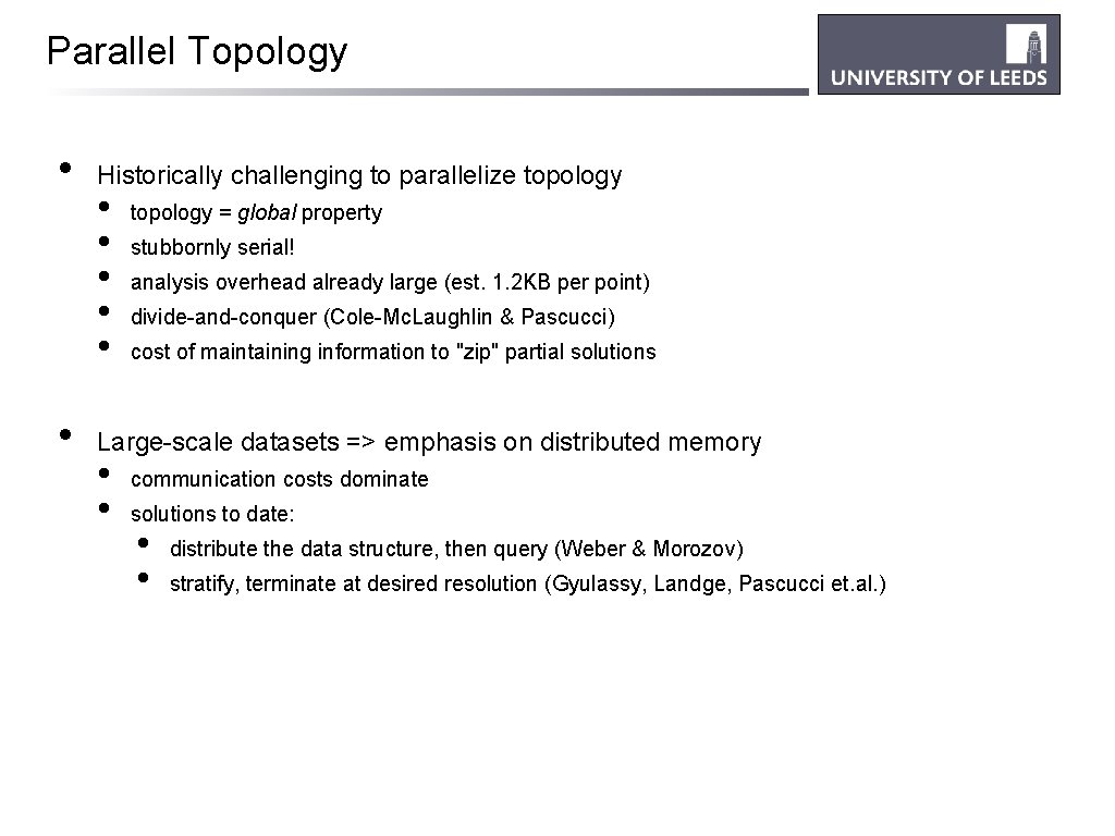
Parallel Topology • • Historically challenging to parallelize topology • • • topology = global property stubbornly serial! analysis overhead already large (est. 1. 2 KB per point) divide-and-conquer (Cole-Mc. Laughlin & Pascucci) cost of maintaining information to "zip" partial solutions Large-scale datasets => emphasis on distributed memory • • communication costs dominate solutions to date: • • distribute the data structure, then query (Weber & Morozov) stratify, terminate at desired resolution (Gyulassy, Landge, Pascucci et. al. )

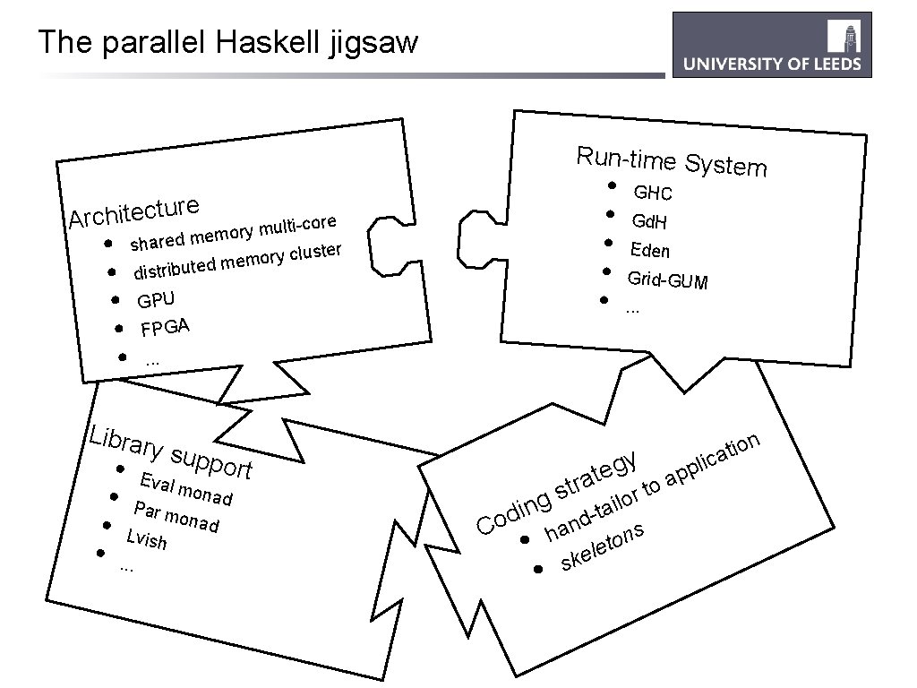
The parallel Haskell jigsaw Run-time System • GHC • Gd. H • Eden • Grid-GUM • . . . e r u t c e t i h Arc • • • ti-core l u m y r o em shared m luster c y r o m e dm distribute GPU FPGA. . . Libra ry su pport • • y g te tra or to s g il n a i t d Eval mona d Par m onad Lvish. . . Co • d n a h ns o t le e k s • l p p a i n o i t ca

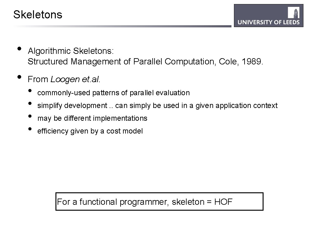
Skeletons • • Algorithmic Skeletons: Structured Management of Parallel Computation, Cole, 1989. From Loogen et. al. • • commonly-used patterns of parallel evaluation simplify development. . can simply be used in a given application context may be different implementations efficiency given by a cost model For a functional programmer, skeleton = HOF

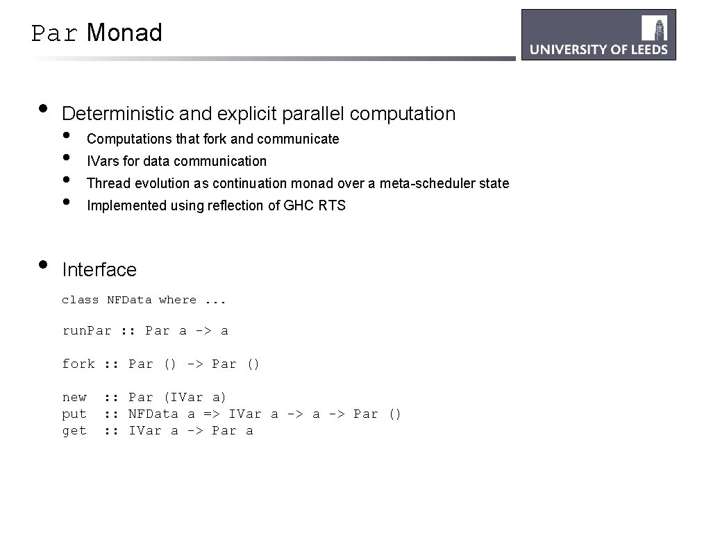
Par Monad • • Deterministic and explicit parallel computation • • Computations that fork and communicate IVars for data communication Thread evolution as continuation monad over a meta-scheduler state Implemented using reflection of GHC RTS Interface class NFData where. . . run. Par : : Par a -> a fork : : Par () -> Par () new put get : : Par (IVar a) : : NFData a => IVar a -> Par () : : IVar a -> Par a

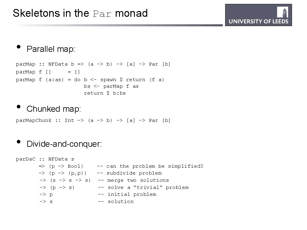
Skeletons in the Par monad • Parallel map: par. Map : : NFData b => (a -> b) -> [a] -> Par [b] par. Map f [] = [] par. Map f (a: as) = do b <- spawn $ return (f a) bs <- par. Map f as return $ b: bs • Chunked map: par. Map. Chunk : : Int -> (a -> b) -> [a] -> Par [b] • Divide-and-conquer: par. Da. C : : => -> -> -> NFData s (p -> Bool) (p -> (p, p)) (s -> s) (p -> s) p s ------- can the problem be simplified? subdivide problem merge two solutions solve a "trivial" problem initial problem solution

Intermission

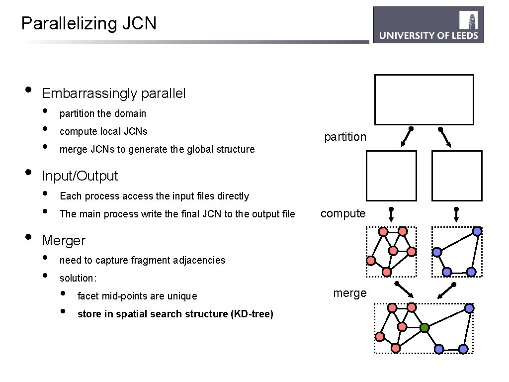
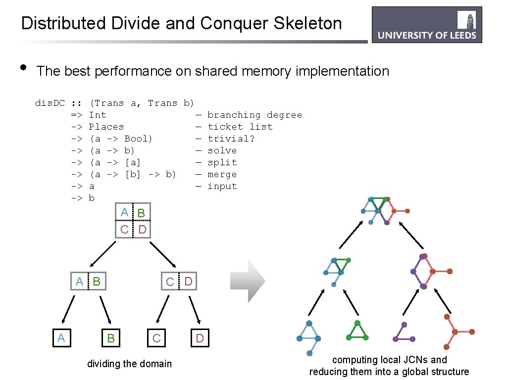
Parallelizing JCN • • • Embarrassingly parallel • • • partition the domain compute local JCNs partition merge JCNs to generate the global structure Input/Output • • Each process access the input files directly The main process write the final JCN to the output file compute Merger • • need to capture fragment adjacencies solution: • • facet mid-points are unique store in spatial search structure (KD-tree) merge

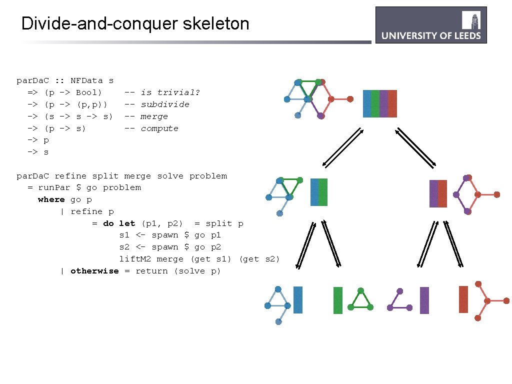
Divide-and-conquer skeleton par. Da. C : : NFData s => (p -> Bool) -> (p, p)) -> (s -> s) -> (p -> s) -> p -> s ----- is trivial? subdivide merge compute par. Da. C refine split merge solve problem = run. Par $ go problem where go p | refine p = do let (p 1, p 2) = split p s 1 <- spawn $ go p 1 s 2 <- spawn $ go p 2 lift. M 2 merge (get s 1) (get s 2) | otherwise = return (solve p)

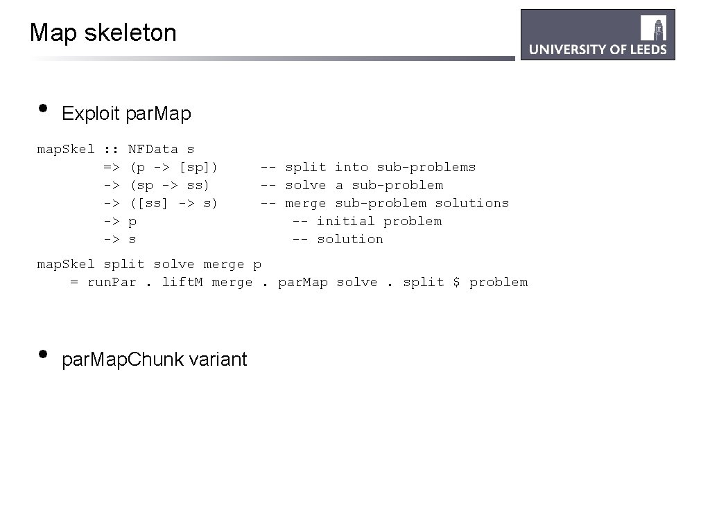
Map skeleton • Exploit par. Map map. Skel : : => -> -> NFData s (p -> [sp]) (sp -> ss) ([ss] -> s) p s -- split into sub-problems -- solve a sub-problem -- merge sub-problem solutions -- initial problem -- solution map. Skel split solve merge p = run. Par. lift. M merge. par. Map solve. split $ problem • par. Map. Chunk variant

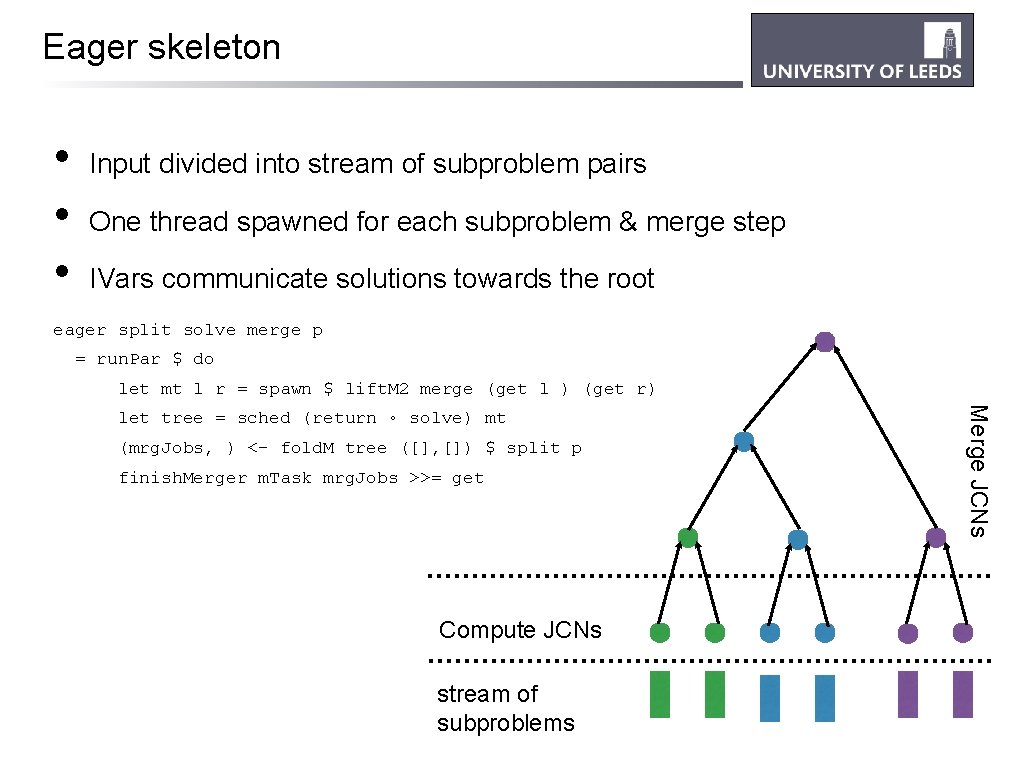
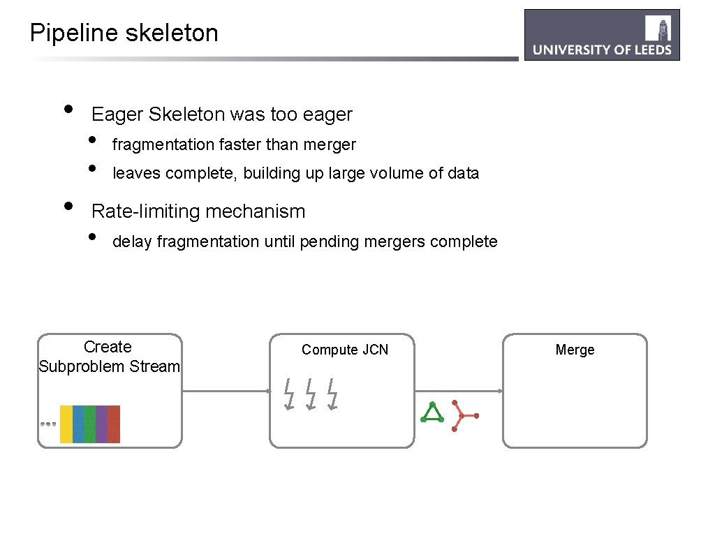
Eager skeleton • • • Input divided into stream of subproblem pairs One thread spawned for each subproblem & merge step IVars communicate solutions towards the root eager split solve merge p = run. Par $ do let mt l r = spawn $ lift. M 2 merge (get l ) (get r) (mrg. Jobs, ) <- fold. M tree ([], []) $ split p finish. Merger m. Task mrg. Jobs >>= get Compute JCNs stream of subproblems Merge JCNs let tree = sched (return ◦ solve) mt

Pipeline skeleton • • Eager Skeleton was too eager • • fragmentation faster than merger leaves complete, building up large volume of data Rate-limiting mechanism • delay fragmentation until pending mergers complete Create Subproblem Stream Compute JCN Merge

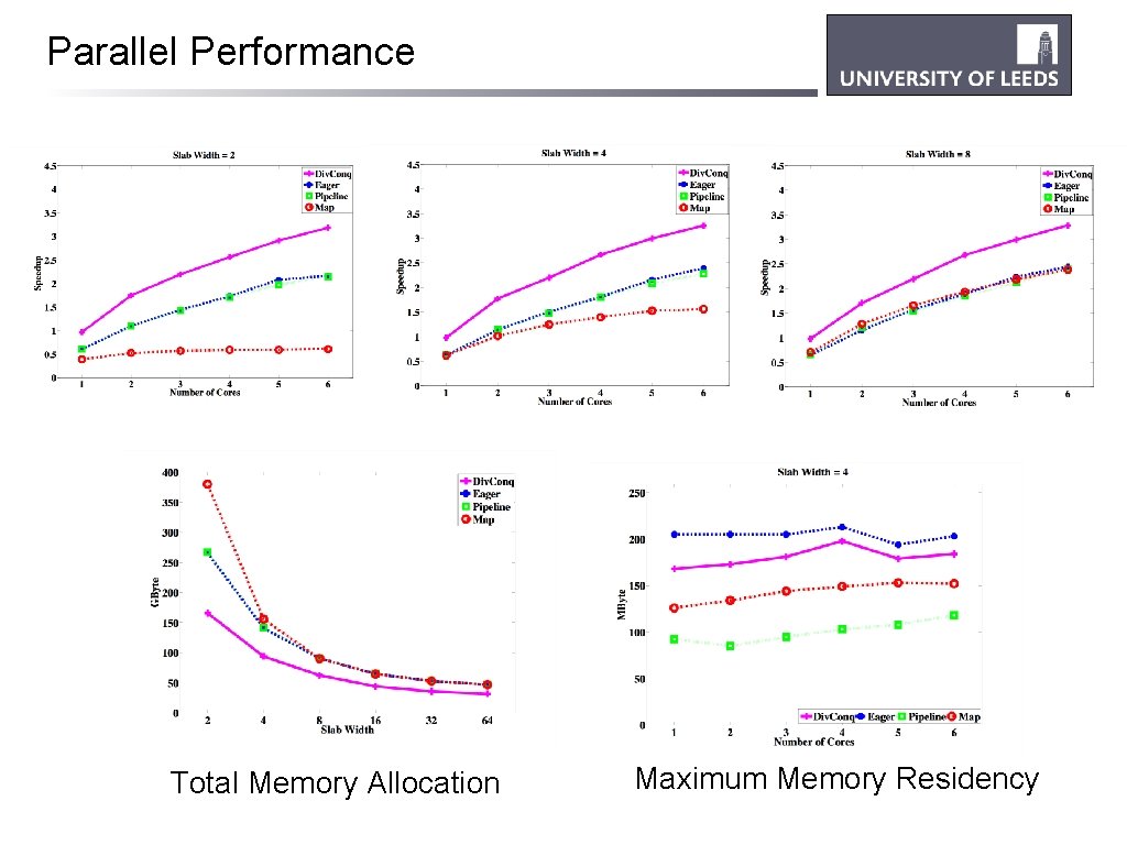
Parallel Performance Total Memory Allocation Maximum Memory Residency

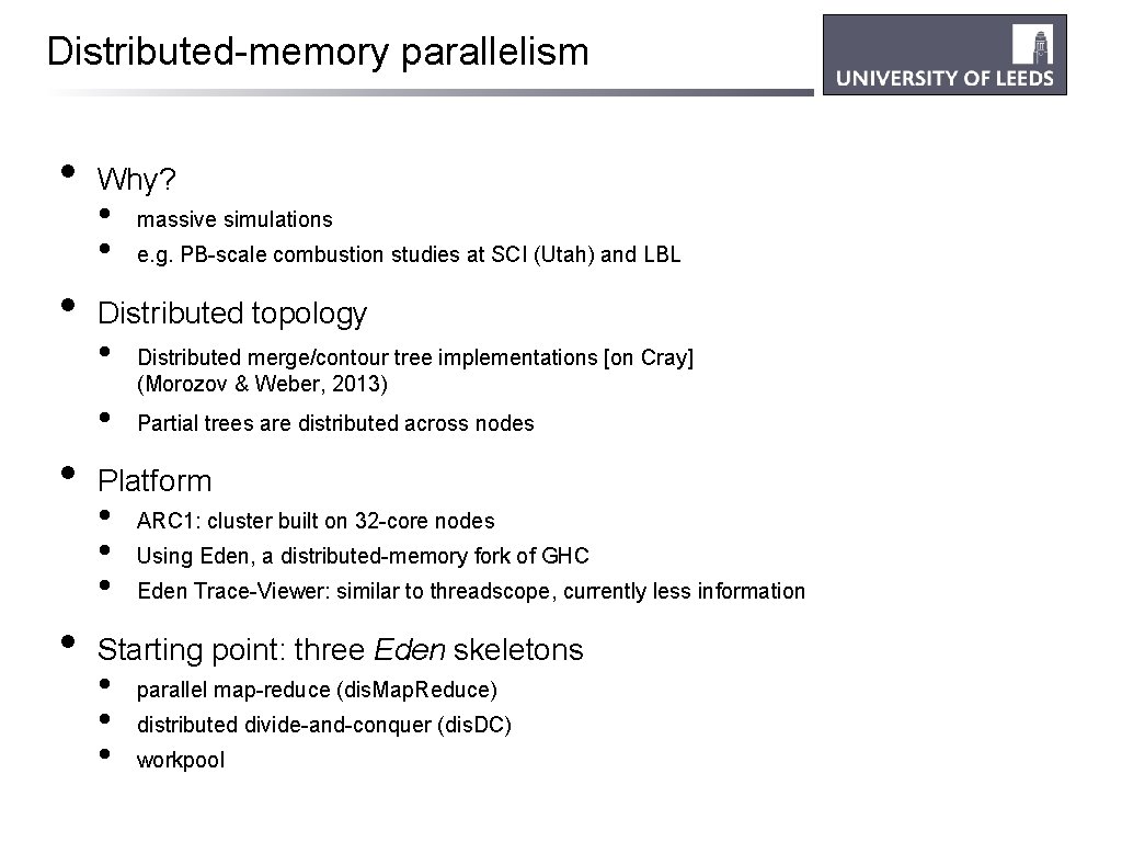
Distributed-memory parallelism • • Why? • • • e. g. PB-scale combustion studies at SCI (Utah) and LBL Distributed topology • • • massive simulations Distributed merge/contour tree implementations [on Cray] (Morozov & Weber, 2013) Partial trees are distributed across nodes Platform • • • ARC 1: cluster built on 32 -core nodes Using Eden, a distributed-memory fork of GHC Eden Trace-Viewer: similar to threadscope, currently less information Starting point: three Eden skeletons • • • parallel map-reduce (dis. Map. Reduce) distributed divide-and-conquer (dis. DC) workpool

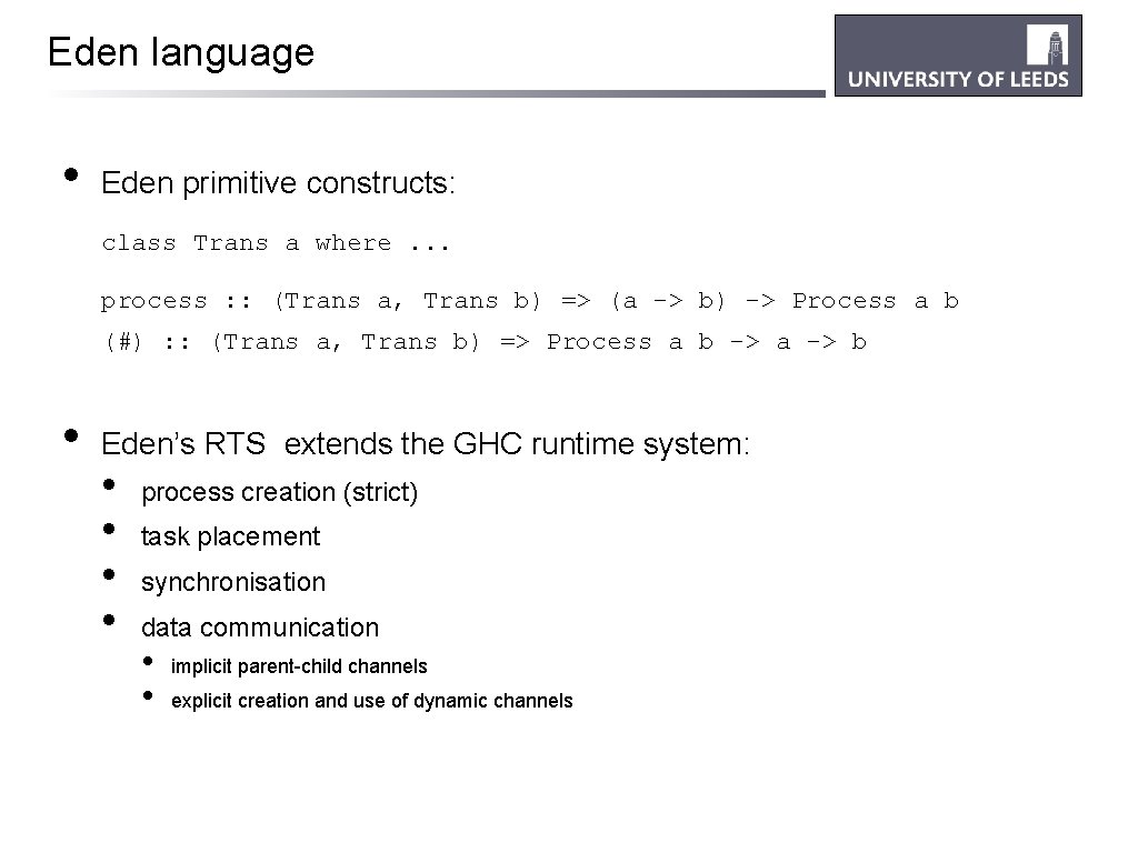
Eden language • Eden primitive constructs: class Trans a where. . . process : : (Trans a, Trans b) => (a -> b) -> Process a b (#) : : (Trans a, Trans b) => Process a b -> a -> b • Eden’s RTS extends the GHC runtime system: • • process creation (strict) task placement synchronisation data communication • • implicit parent-child channels explicit creation and use of dynamic channels

Eden skeletons • Map-reduce: map : : (a -> b) -> [a] -> [b] foldr : : (b -> c) -> c -> [b] -> c map. Redr : : (b -> c) -> c -> (a -> b) -> [a] -> c map. Redr rf e mf = (foldr rf e). (map mf) • Distributed map-reduce: dis. Map : : (Trans a, Trans b) -> (a -> b) -> [a] -> [b] dis. Map. Redr : : dis. Map. Redr rf | no. Pe == 1 | otherwise (Trans a, Trans b) => (b -> b) -> b -> (a -> b)->[a] -> b e mf xs = map. Redr g e f xs = (foldr rf e). (dis. Map. Redr rf e mf)). (split. Into. N no. Pe) $ xs

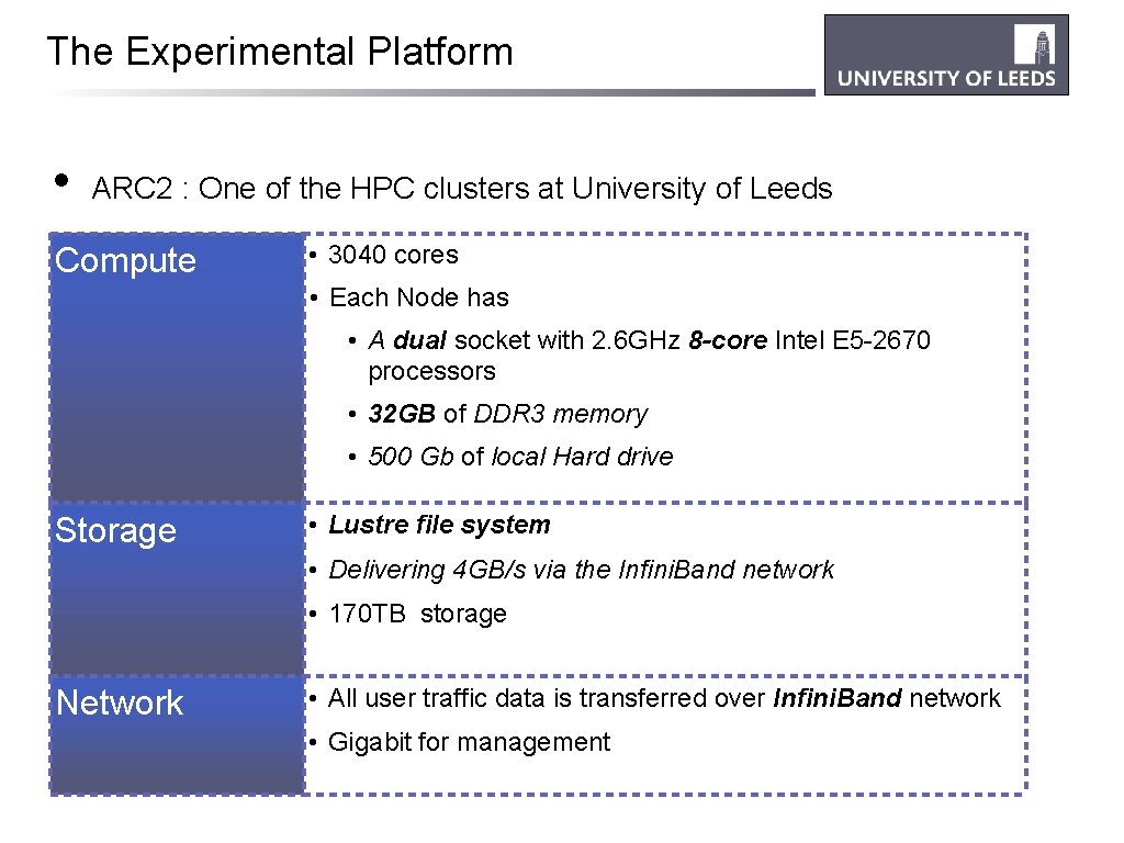
The Experimental Platform • ARC 2 : One of the HPC clusters at University of Leeds Compute • 3040 cores • Each Node has • A dual socket with 2. 6 GHz 8 -core Intel E 5 -2670 processors • 32 GB of DDR 3 memory • 500 Gb of local Hard drive Storage • Lustre file system • Delivering 4 GB/s via the Infini. Band network • 170 TB storage Network • All user traffic data is transferred over Infini. Band network • Gigabit for management

Distributed Divide and Conquer Skeleton • The best performance on shared memory implementation dis. DC : : => -> -> (Trans a, Trans b) Int — branching degree Places — ticket list (a -> Bool) — trivial? (a -> b) — solve (a -> [a] — split (a -> [b] -> b) — merge a — input b A B C D A B A C D B C dividing the domain D computing local JCNs and reducing them into a global structure

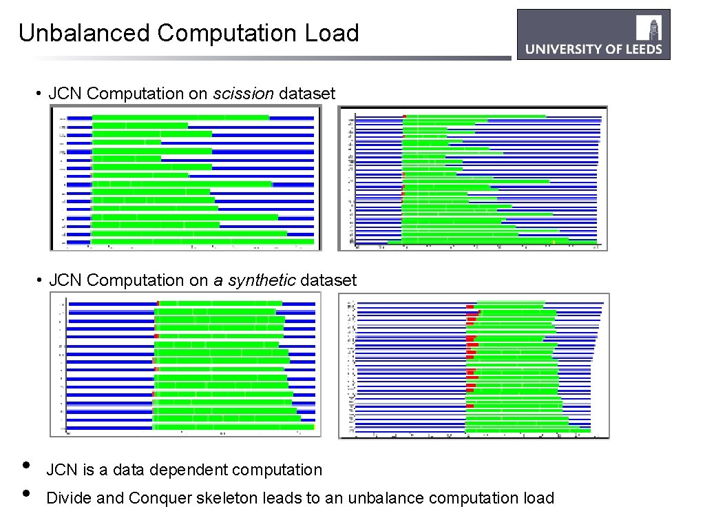
Unbalanced Computation Load • JCN Computation on scission dataset • JCN Computation on a synthetic dataset • • JCN is a data dependent computation Divide and Conquer skeleton leads to an unbalance computation load

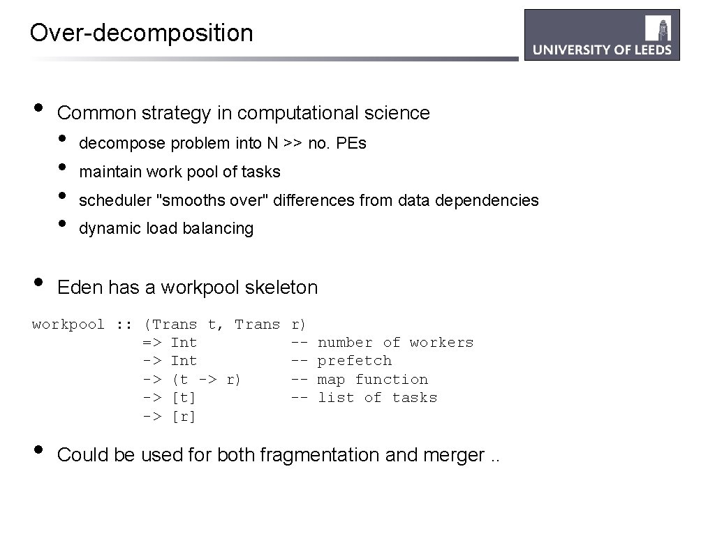
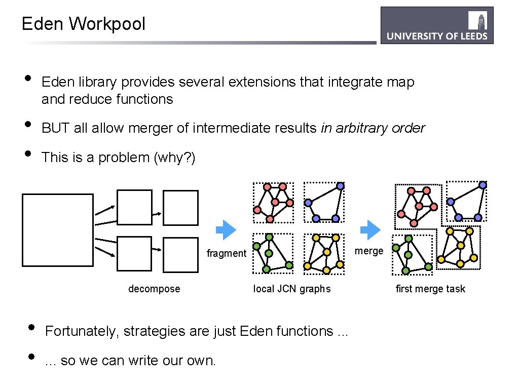
Over-decomposition • • Common strategy in computational science • • decompose problem into N >> no. PEs maintain work pool of tasks scheduler "smooths over" differences from data dependencies dynamic load balancing Eden has a workpool skeleton workpool : : (Trans t, Trans => Int -> (t -> r) -> [t] -> [r] • r) ----- number of workers prefetch map function list of tasks Could be used for both fragmentation and merger. .

Eden Workpool • • • Eden library provides several extensions that integrate map and reduce functions BUT allow merger of intermediate results in arbitrary order This is a problem (why? ) merge fragment decompose • • local JCN graphs Fortunately, strategies are just Eden functions. . . so we can write our own. first merge task

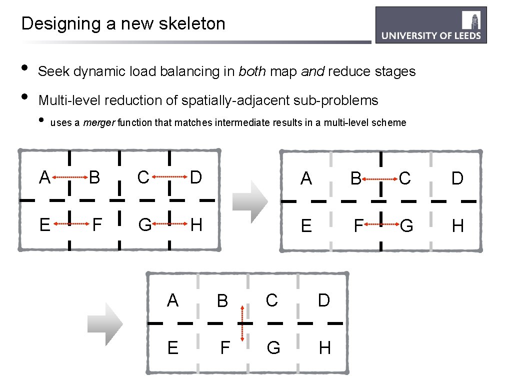
Designing a new skeleton • • Seek dynamic load balancing in both map and reduce stages Multi-level reduction of spatially-adjacent sub-problems • uses a merger function that matches intermediate results in a multi-level scheme A B C D E F G H

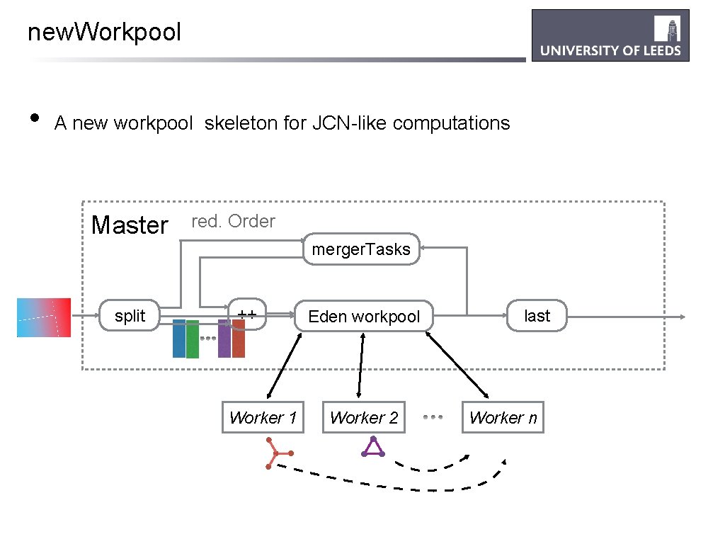
new. Workpool • A new workpool skeleton for JCN-like computations Master red. Order merger. Tasks split ++ Worker 1 Eden workpool Worker 2 last Worker n

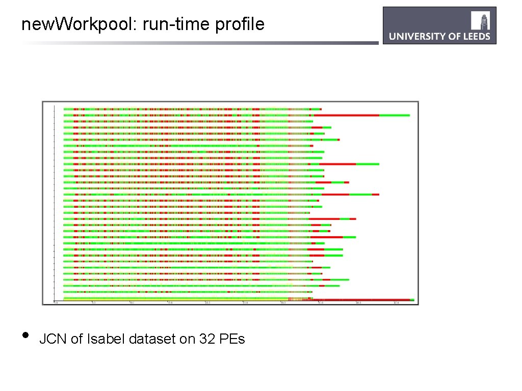
new. Workpool: run-time profile • JCN of Isabel dataset on 32 PEs

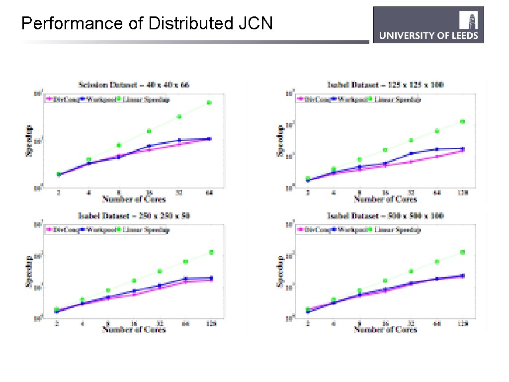
Performance of Distributed JCN

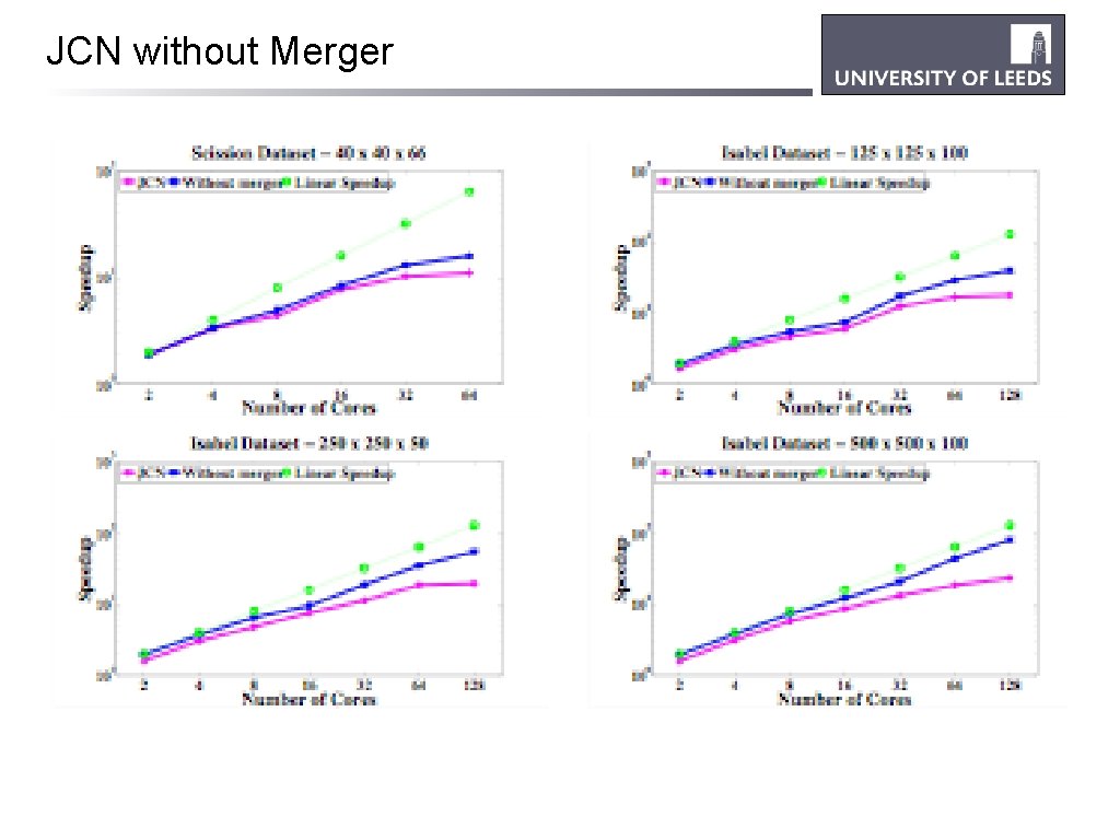
JCN without Merger

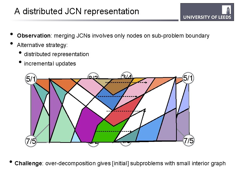
A distributed JCN representation • • Observation: merging JCNs involves only nodes on sub-problem boundary Alternative strategy: • distributed representation • incremental updates 5/1 8/3 3/4 5/1 7/5 6/2 4/3 7/5 • Challenge: over-decomposition gives [initial] subproblems with small interior graph

Speedup Shared & Distributed Mem Implementation Number of Cores

What we achieved / found. . . • Unexpected lessons on skeletons • • • skeletons can themselves be non-trivial functions conveniently abstract for straightforward cases inconveniently abstract for understanding performance can we have our cake and eat it too? … are there sensible building blocks for skeletons? • Tooling still an issue • • • Peter Wortmann's enhanced profiling support invaluable - but further work needed (see Haskell Symposium 2013 paper) hard to measure communication costs profiling over 100's of cores integrating IO into skeletons and distributed Haskell Contributions • • • scaled parallel JCN implementation from small to modest datasets understood issues affecting further scaling achieved some impact. . .

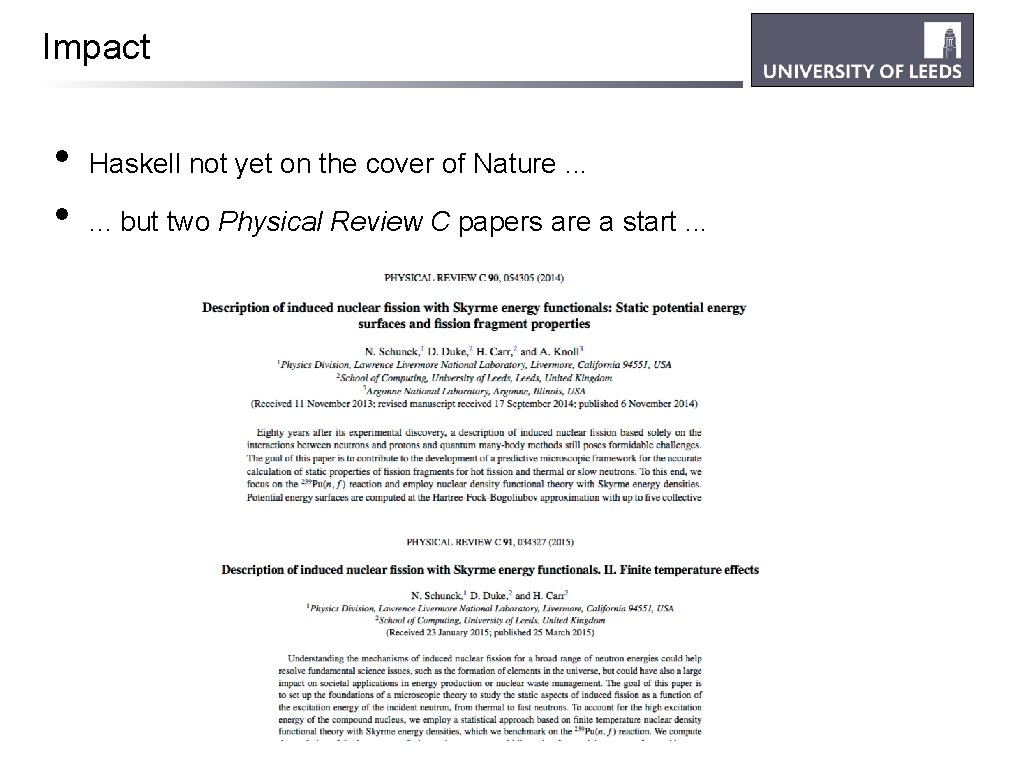
Impact • • Haskell not yet on the cover of Nature. . . but two Physical Review C papers are a start. . .

Broader issues • • • So why isn't Haskell used in. . • • • . . computational science (Fortran, C/C++, Chapel, Open. CL, . . . ). . computer graphics & games (C++, . . . ). . <insert your favourite application area>? Technology • • • technology only just mature absence of a standard (who programs in Haskell'98 these days? !) tools, esp. cost modelling and profiling legacy code and inertia different engineering challenges and trade-offs from success areas People issues • • • Your top C++ programmer leaves. . . replace in days Your top (HPC) Haskell programmer leaves. . . replace when? Project risk against likely benefits

What we achieved. . . • Contributions • • scaled parallel JCN implementation from small to modest datasets understood issues affecting further scaling • Unexpected lessons on skeletons • • • skeletons can themselves be non-trivial functions conveniently abstract for straightforward cases inconveniently abstract for understanding performance can we have our cake and eat it too? … are there sensible building blocks for skeletons? • Tooling still an issue • • e. g. measuring communication costs, profiling over 100 s of cores, IO Ongoing and future work • • moving work towards GPU clusters heterogeneous resources, complex memory hierarchy in-situ processing run on Tianhe-2 ? !

Future • • Challenges • • • Haskell / FP have made inroads in some sectors Why? What do they excel at? EDSLs - Obsidian, Repa, Accelerate. . . Heterogeneous resources, complex memory hierarchy In-situ processing Try running on Tianhe-2 ? ! Current plans • • Memory-sensitive representation Games - one of the most performance-critical CS applications

Acknowledgements • UK Engineering and Physical Sciences Research Council Multifield Extension of Topological Analysis, Grant EP/J 013072/1 • Collaborators and contributors • Fouzhan Hosseini • Nicholas Schunck • Hamish Carr • Geng Zhao • Amit Chattopadhyay • Aaron Knoll • Jost Berthold • Thomas Horstmeyer • Hans-Wolfgang Loidl • Ben Lippmeier