Single Function QuineMc Cluskey 2 Level Minimization Shantanu

Single Function Quine-Mc. Cluskey 2 -Level Minimization Shantanu Dutt University of Illinois at Chicago Acknowledgement: Transcribed to Powerpoint by Huan Ren from Prof. Shantanu Dutt’s handwritten notes (later added to significantly by Shantanu Dutt)

Basic Two-Level Minimization Steps The basic steps are the same for K-Map and Quine Mc. Cluskey (QM): 1. Form all PIs 2. Determine a minimum cost set of PIs to cover all minterms (MTs) a) Determine EPIs, include them in the final expression and delete all MTs they cover b) Determine a min cost set of the remaining PIs to cover the remaining MTs. This is a really hard problem—NP-hard, i. e. , to solve it optimally it takes a worst-case computation time that is exponential in the # of nonessential PIs.

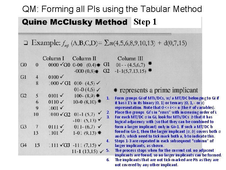
QM: Forming all PIs using the Tabular Method Step 1 G 0 G 1 G 2 G 1 1. G 2 G 3 2. 3. 4. 5. 6. Form groups Gi of MTs/DCs, w/ a MT/DC belonging to Gi if it has i 1’s in its binary (0, 1) or ternary (0, 1, - or x) representation. Note that 0 <= i <= n (the # of variables). Place the groups Gi’s in “rows” with increasing order of i. For each MT/DC a in Gi, look for MTs/DCs b that it has logical adjacency with (so that they can be combined to form a larger implicant) only in Gi+1. If such a MT/DC b found in Gi+1, then the larger implicant (a, b) covers both a and b, which need to tick mark both a, b to indicate this. Steps 1 -3 are repeated in each subsequent “column” of larger implicants, as shown. The process stops when for the current col. no adjacent implicants are found, so no larger implicants can be formed. The implicants that are not tick-marked are PIs as they are not covered by any other implicant.

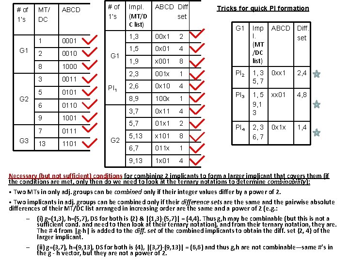
# of 1’s G 1 G 2 G 3 MT/ DC ABCD 1 0001 2 0010 8 1000 3 0011 5 0101 6 0110 9 1001 7 0111 13 1101 # of 1’s G 1 PI 1 G 2 Impl. (MT/D C list) ABCD Diff. set 1, 3 00 x 1 2 1, 5 0 x 01 4 1, 9 x 001 8 2, 3 001 x 1 2, 6 0 x 10 4 8, 9 100 x 1 3, 7 0 x 11 4 5, 7 01 x 1 2 5, 13 x 101 8 6, 7 011 x 1 9, 13 1 x 01 4 Tricks for quick PI formation G 1 Imp l. (MT /DC list) ABCD Diff. set PI 2 1, 3 5, 7 0 xx 1 2, 4 PI 3 1, 5 9, 1 3 xx 01 4, 8 PI 4 2, 3 6, 7 0 x 1 x 1, 4 Necessary (but not sufficient) conditions for combining 2 implicants to form a larger implicant that covers them (if the conditions are met, only then do we need to look at the ternary notations to determine combinability): • Two MTs in only adj. groups can be combined only if their integer values differ by a power of 2. • Two implicants in adj. groups can be combined only if their difference sets are the same and the pairwise absolute differences of their MT/DC list arranged in increasing order are the same and a power of 2 (e. g. : – – (i) g=(1, 3), h=(5, 7), DS for both is {2} & |(1, 3)-(5, 7)| = (4, 4). Thus g, h may be combinable (but this is not a sufficient cond. and need to then look at their ternary notation), and from their ternary notation, they are. The # 4 from |g-h| is added to the diff. set of the combined implicants to obtain the diff. set {2, 4} of the larger implicant. (ii) g=(3, 7), h=(9, 13), DS for both is {4}, |(3, 7)-(9, 13)| = (6, 6) and thus g, h are not combinable—same #’s in the g - h vector, but they are not a power of 2.

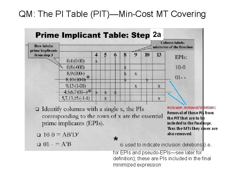
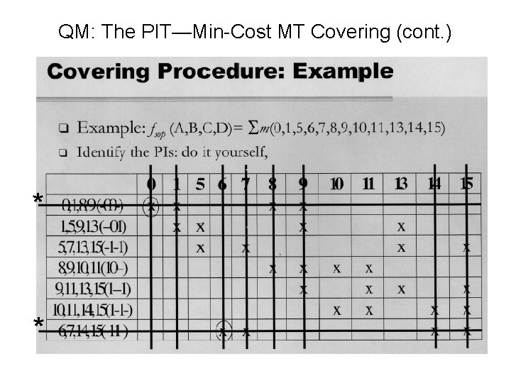
QM: The PI Table (PIT)—Min-Cost MT Covering 2 a * Inclusion removal/deletion: Removal of those PIs from the PIT that are to be included in the final expr. Thus the MTs they cover are also removed. is used to indicate inclusion deletions (i. e. for EPIs and pseudo-EPIs—see later for definition); these are PIs included in the final minimized expression

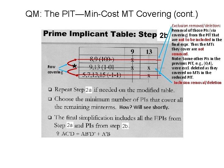
QM: The PIT—Min-Cost MT Covering (cont. ) 2 b Row covering * 2 a How? Will see shortly. 2 a 2 b Exclusion removal/deletion: Removal of those PIs (via covering) from the PIT that are not to be included in the final expr. Thus the MTs they cover are not removed. Note: Some other PIs in the previous PIT, e. g. , (0, 4), were excl. deleted as they covered no MTs in the reduced PIT. Inclusion removal/deletion

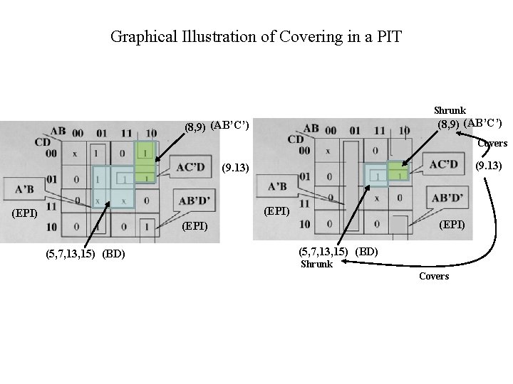
Graphical Illustration of Covering in a PIT Shrunk (8, 9) (AB’C’) Covers (9. 13) (EPI) (5, 7, 13, 15) (BD) Shrunk Covers

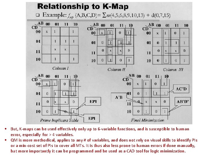
• But, K-maps can be used effectively only up to 6 -variable functions, and is susceptible to human error, especially for > 4 variables. • QM is more methodical, applies to any # of variables, and does not rely on visual skills to identify PIs or a min-cost set of PIs to cover all MTs. It is thus also less prone to human errors if done manually, but more importantly it can be programmed and be used as a CAD tool for logic minimization.

QM: The PIT—Min-Cost MT Covering (cont. ) * *

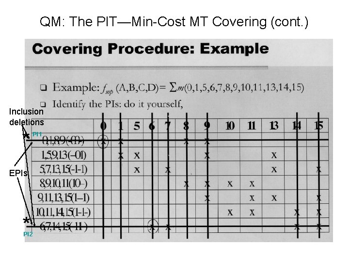
QM: The PIT—Min-Cost MT Covering (cont. ) Inclusion deletions * EPIs * PI 2 PI 1

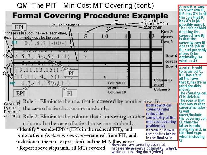
QM: The PIT—Min-Cost MT Covering (cont. ) Exclusion deletions In these cases both PIs cover each other, But that may not always be the case PI 1 C Covering by one MT/col of another A row Ri is said to cover row Rj, if Ri has X’s in all the cols that Rj has X’s in (& possibly more). The idea behind deleting the covered row Rj is that the covering row Ri does the job of Rj, and probably more. Q for optimality: At what cost? A col Ci is said to cover col Cj, C if Ci has X’s in all the rows that Cj has X’s in PI 2 (and possibly more). The covering col. Ci is deleted. The idea is that any PI that Covering Both row & col covers/includes by one covering rules Cj will PI/row of reduce the cover/include another complexity of the covering col. min-cost covering Ci; thus the latter is autoproblem by • Identify “pseudo-EPIs” (EPIs in the reduced PIT), and narrowing down matically incl. in the choices for PIs the final expr. remove them (inclusion removal—removal from PIT, and when including in the final SOP. Cj inclusion in the min. expression) and the MTs. However they cover. row-covering does not • Repeat above steps until all MTs covered necessarily preserve optimality (why? ), while col-covering does (why? )

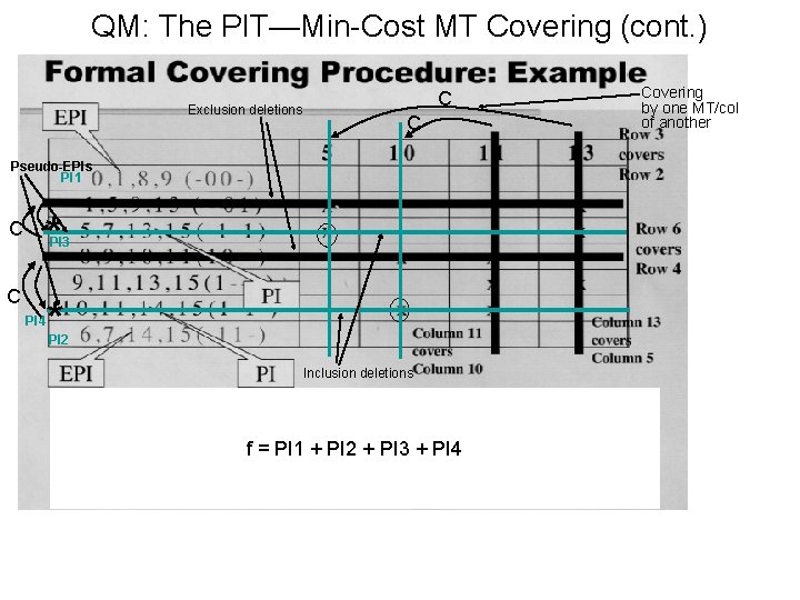
QM: The PIT—Min-Cost MT Covering (cont. ) Exclusion deletions C C Pseudo-EPIs PI 1 C C * PI 3 * PI 4 PI 2 Inclusion deletions f = PI 1 + PI 2 + PI 3 + PI 4 Covering by one MT/col of another

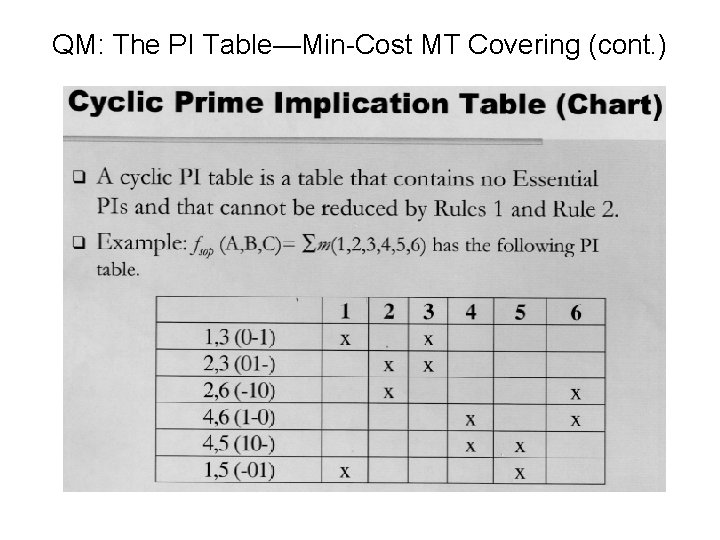
QM: The PI Table—Min-Cost MT Covering (cont. )

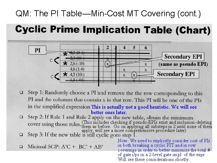
QM: The PI Table—Min-Cost MT Covering (cont. ) * C C * * * (same as pseudo EPI) (for incl. removal) This is actually a good heuristic. We will see can Betternot heuristics than random choice better onesbelater. used, as shown in subsequent slides (This includes checking if pseudo-EPIs exist and inclusion-deleting them as before. Go on applying all substeps in 2 until none of them apply; will see a more comprehensive procedure later) Note: We need to explicitly consider cost of PIs in both breaking a cyclic PIT and in row coverings in order to better minimize the total # of gate i/ps in a 2 -level gate impl. of the expr. Will see these considerations shortly.

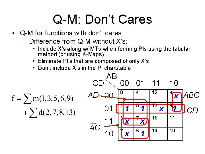
Q-M: Don’t Cares • Q-M for functions with don’t cares: – Difference from Q-M without X’s: • Include X’s along w/ MTs when forming PIs using the tabular method (or using K-Maps) • Eliminate PI’s that are composed of only X’s • Don’t include X’s in the PI chart/table AB CD 00 01 11 4 12 AD 00 0 AC 01 1 11 3 10 2 1 5 x 7 x 6 10 8 x ABC 9 1 1 13 x 15 11 1 14 10 x CD

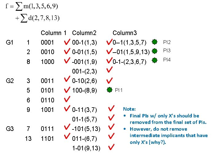
G 1 Column 2 Column 3 1 0001 00 -1(1, 3) 0 --1(1, 3, 5, 7) PI 2 2 0010 0 -01(1, 5) --01(1, 5, 9, 13) PI 3 8 1000 -001(1, 9) 0 -1 -(2, 3, 6, 7) PI 4 001 -(2, 3) G 2 3 0011 0 -10(2, 6) 5 0101 100 -(8, 9) 6 0110 9 1001 0 -11(3, 7) 01 -1(5, 7) G 3 7 0111 -101(5, 13) 13 1101 011 -(6, 7) 1 -01(9, 13) PI 1 Note: • Final PIs w/ only X’s should be removed from the final set of Pis. • However, do not remove intermediate implicants that have only X’s (why? ).

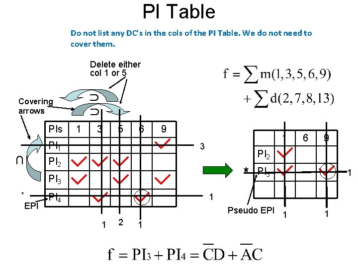
PI Table Do not list any DC’s in the cols of the PI Table. We do not need to cover them. Delete either col 1 or 5 ∩ ∩ Covering arrows PIs 1 3 5 6 PI 1 ∩ 9 1 3 * PI 3 EPI PI 4 9 PI 2 * 6 PI 3 1 1 1 2 Pseudo EPI 1 1 1

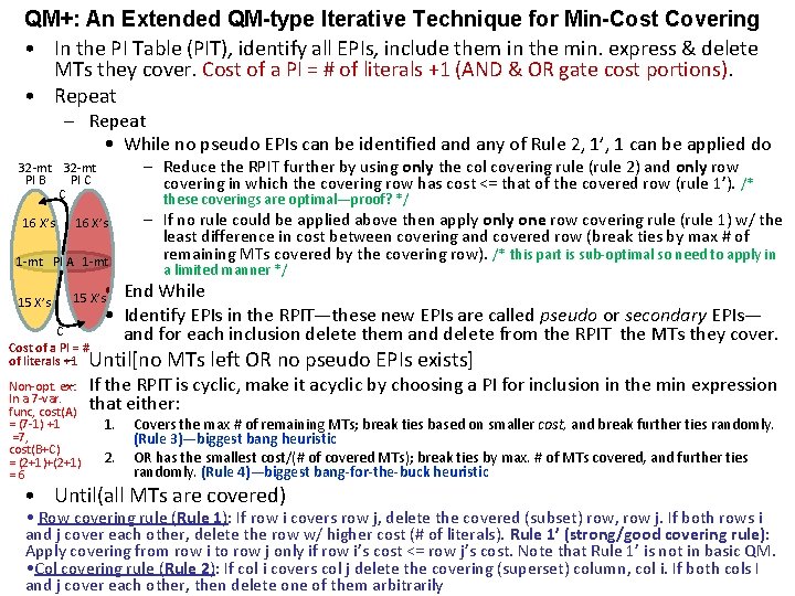
QM+: An Extended QM-type Iterative Technique for Min-Cost Covering • In the PI Table (PIT), identify all EPIs, include them in the min. express & delete MTs they cover. Cost of a PI = # of literals +1 (AND & OR gate cost portions). • Repeat – Repeat • While no pseudo EPIs can be identified any of Rule 2, 1’, 1 can be applied do – Reduce the RPIT further by using only the col covering rule (rule 2) and only row covering in which the covering row has cost <= that of the covered row (rule 1’). /* 32 -mt PI B PI C C 16 X’s these coverings are optimal—proof? */ 16 X’s 1 -mt PI A 1 -mt 15 X’s • C Cost of a PI = # of literals +1 – If no rule could be applied above then apply one row covering rule (rule 1) w/ the least difference in cost between covering and covered row (break ties by max # of remaining MTs covered by the covering row). /* this part is sub-optimal so need to apply in a limited manner */ End While • Identify EPIs in the RPIT—these new EPIs are called pseudo or secondary EPIs— and for each inclusion delete them and delete from the RPIT the MTs they cover. – Until[no MTs left OR no pseudo EPIs exists] Non-opt. ex: – In a 7 -var. func, cost(A) = (7 -1) +1 =7, cost(B+C) = (2+1)+(2+1) =6 If the RPIT is cyclic, make it acyclic by choosing a PI for inclusion in the min expression that either: 1. 2. Covers the max # of remaining MTs; break ties based on smaller cost, and break further ties randomly. (Rule 3)—biggest bang heuristic OR has the smallest cost/(# of covered MTs); break ties by max. # of MTs covered, and further ties randomly. (Rule 4)—biggest bang-for-the-buck heuristic • Until(all MTs are covered) • Row covering rule (Rule 1): If row i covers row j, delete the covered (subset) row, row j. If both rows i and j cover each other, delete the row w/ higher cost (# of literals). Rule 1’ (strong/good covering rule): Apply covering from row i to row j only if row i’s cost <= row j’s cost. Note that Rule 1’ is not in basic QM. • Col covering rule (Rule 2): If col i covers col j delete the covering (superset) column, col i. If both cols I and j cover each other, then delete one of them arbitrarily

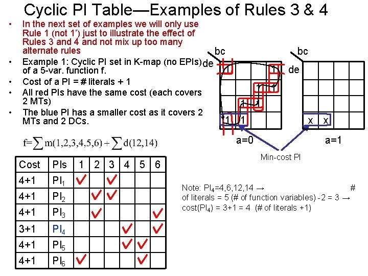
Cyclic PI Table—Examples of Rules 3 & 4 • • • In the next set of examples we will only use Rule 1 (not 1’) just to illustrate the effect of Rules 3 and 4 and not mix up too many alternate rules bc Example 1: Cyclic PI set in K-map (no EPIs) de 1 of a 5 -var. function f. Cost of a PI = # literals + 1 All red PIs have the same cost (each covers 2 MTs) The blue PI has a smaller cost as it covers 2 1 MTs and 2 DCs. bc 1 de 1 1 1 x a=0 Cost PIs 4+1 PI 1 4+1 PI 2 4+1 PI 3 3+1 PI 4 4+1 PI 5 4+1 PI 6 1 2 3 4 5 6 x a=1 Min-cost PI Note: PI 4=4, 6, 12, 14 → # of literals = 5 (# of function variables) -2 = 3 → cost(PI 4) = 3+1 = 4 (# of literals +1)

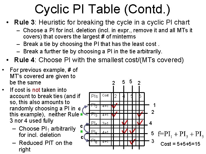
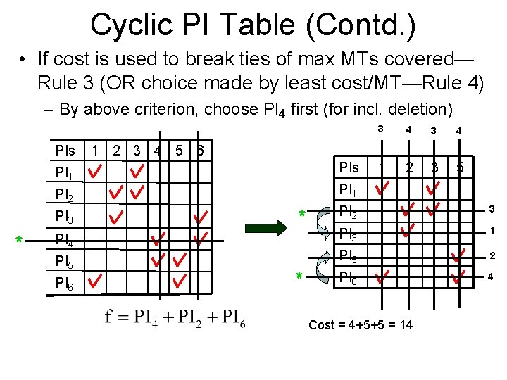
Cyclic PI Table (Contd. ) • Rule 3: Heuristic for breaking the cycle in a cyclic PI chart – Choose a PI for incl. deletion (incl. in expr. , remove it and all MTs it covers) that covers the largest # of minterms – Break a tie by choosing the PI that has the least cost. – Break a further tie by choosing a PI in the tie arbitrarily. • Rule 4: Choose PI with the smallest cost/(MTs covered) • For previous example, # of MT’s covered are given to be the same • If cost is not taken into account to break ties (and if so, this also amounts to randomly choosing a PI in c this example), neither Rule* 3 nor 4 used fully – Choose PI 1 arbitrarily c *c for incl. deletion – Reduced PIT on the right 2 5 5 2 4 6 PIs Cost PI 2 4+1 PI 3 4+1 PI 4 3+1 PI 5 4+1 5 PI 6 4+1 3 2 5 1 2 4 Cost = 5+5+5=15

Cyclic PI Table (Contd. ) • If cost is used to break ties of max MTs covered— Rule 3 (OR choice made by least cost/MT—Rule 4) – By above criterion, choose PI 4 first (for incl. deletion) PIs * PI 4 PI 5 PI 6 3 4 1 2 3 5 PI 1 PI 2 * 4 1 2 3 4 5 6 PI 1 PI 3 3 * PI 2 3 PI 3 1 PI 5 2 PI 6 4 Cost = 4+5+5 = 14

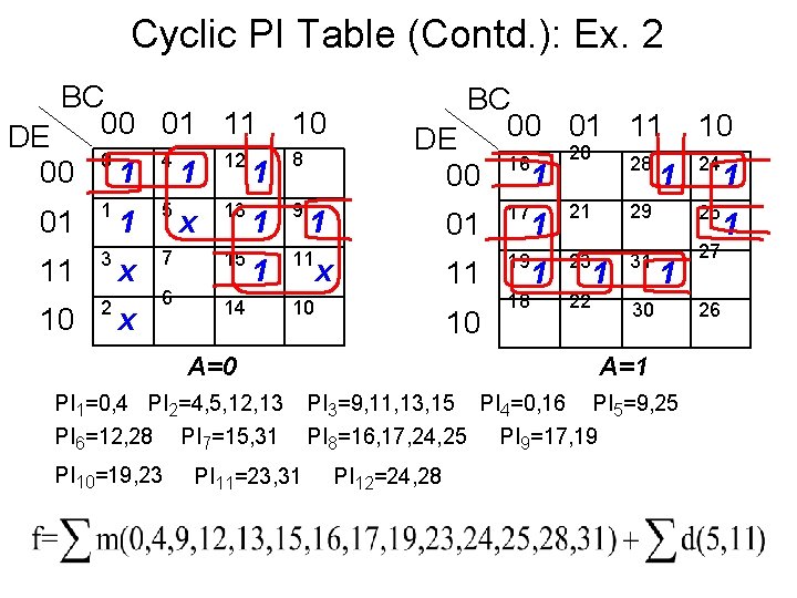
Cyclic PI Table (Contd. ): Ex. 2 BC 00 01 11 10 DE 8 0 4 12 00 1 1 1 01 1 11 3 10 2 1 5 x 7 15 6 14 x x 13 1 9 1 11 BC 00 01 11 10 DE 20 16 28 00 1 1 241 1 x 10 PI 10=19, 23 PI 11=23, 31 17 11 19 10 A=0 PI 1=0, 4 PI 2=4, 5, 12, 13 PI 6=12, 28 PI 7=15, 31 01 18 1 21 29 25 1 23 31 27 22 1 1 30 A=1 PI 3=9, 11, 13, 15 PI 4=0, 16 PI 5=9, 25 PI 8=16, 17, 24, 25 PI 9=17, 19 PI 12=24, 28 26 1

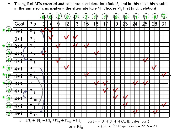
• Taking # of MTs covered and cost into consideration (Rule 3, and in this case this results in the same soln. as applying the alternate Rule 4): Choose PI 8 first (incl. deletion) Cost PIs * 6 PI 1 3+1 PI 2 7 3+1 PI 3 2 4+1 PI 4 5 4+1 PI 5 * 8 * 11 * 1 4+1 PI 6 4+1 PI 7 3+1 PI 8 3 4+1 PI 9 9 4+1 PI 10 10 4+1 PI 11 4+1 PI 12 * 4 7 8 7 0 4 9 12 13 4+1 * 6 PI 3 7 1 1 9 9 1 1 8 11 6 15 16 17 19 23 24 25 28 31 cost = 4+3+4+4 (AND gates’ cost) + 6 (6 PIs OR gate cost) = 22+6 = 28

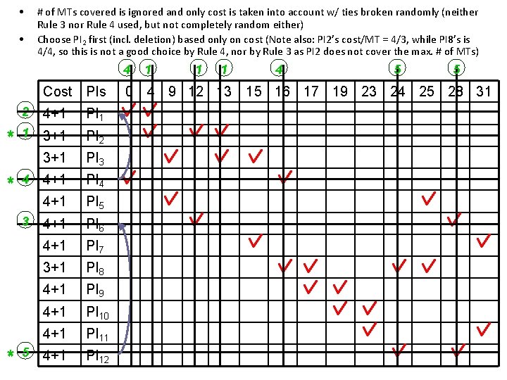
• • # of MTs covered is ignored and only cost is taken into account w/ ties broken randomly (neither Rule 3 nor Rule 4 used, but not completely random either) Choose PI 2 first (incl. deletion) based only on cost (Note also: PI 2’s cost/MT = 4/3, while PI 8’s is 4/4, so this is not a good choice by Rule 4, nor by Rule 3 as PI 2 does not cover the max. # of MTs) 4 Cost PIs * * 2 4+1 PI 1 1 3+1 PI 2 3+1 PI 3 4+1 PI 4 4+1 PI 5 4+1 PI 6 4+1 PI 7 3+1 PI 8 4+1 PI 9 4+1 PI 10 4+1 PI 11 4+1 PI 12 4 3 * 5 1 1 1 0 4 9 12 13 4 5 5 15 16 17 19 23 24 25 28 31

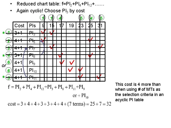
• Reduced chart table: f=PI 2+PI 4+PI 12+…… • Again cyclic! Choose PI 3 by cost 1 Cost PIs * * or * 1 3+1 PI 3 2 4+1 PI 5 3 4+1 PI 7 4 3+1 PI 8 6 4+1 PI 9 6 4+1 PI 10 5 4+1 PI 11 1 4 5 9 15 17 19 23 25 31 This cost is 4 more than when using # of MTs as the selection criteria in an acyclic PI table

Time-Complexity of QM • Let p be the # of PIs and m the # of MTs in an n-variable function • # of iterations of QM (each iter. consists of EPIs/p-EPIs incl. deletion or application of rules 1 or 2): In each iteration at least 1 col or row is deleted (incl. or excl. deletions). Thus # of worst-case iterations is O(p+m) = O(max(p, m)) (note could be Q(max(p, m)) but more analysis needed for that). • Each iteration takes Q(max(m*p 2, p*m 2)) time due to worst-case of all pair-wise comparisons among rows and cols to determine row and col coverings, and Q(m*p) to determine EPIs (or psuedo-EPIs). • Thus total time complexity is O(max(p, m))*(max(m*p 2 , p*m 2))) = O(max(m*p 3, p 2*m 2, p*m 3)) = O(max(m*p 3, p*m 3)), since if p < m, then p*m 3 > p 2*m 2, else (p >= m) m*p 3 >= p 2*m 2 • What are the worst case values of p and m as functions of n?

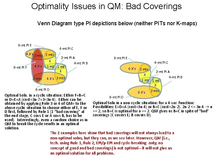
Optimality Issues in QM: Bad Coverings Venn Diagram type PI depictions below (neither PITs nor K-maps) 8 -mt PI E 4 -mt PI C 4 X’s 2 mts X 8 -mt PI F 4 X’s 2 mts 2 -mt PI A 1 mt X 4 X’s 2 mts 8 -mt PI D 8 -mt PI E 4 -mt PI C 4 -mt PI B 6 X’s 2 mts X 1 mt 6 X’s 2 -mt PI A 1 mt X 2 mts 4 -mt PI B Optimal Soln. in a cyclic situation: Either F+B+C 8 -mt PI D or D+E+A (cost=3 n-7+3=3 n-4). Either can be Optimal Soln in a non-cyclic situation: for a 4 -var. function: obtained by applying Rule 3 or 4 of QM+ to the above cyclic situation to choose either of E, F or Possibilities: E+D+A (cost=3 n-4) or B+C (cost=2 n-2). 2 n-2 <= 3 n-4 n >= 2, so B+C is optimal for n >= 2. QM gives us B+C in spite of “bad” D first, followed by Rule 1 (1 “bad covering” at coverings (C covers E; B covers D). the end stage, C covs E or A covs B, has to be used). Interestingly, even a random choice as in QM to break the cycle results in an optimal solution. The 2 examples here show that bad coverings will not always lead to a non-optimal solns, but they can, as we see later. However, QM (i. e. , tech. using Rule 1, Rule 2, EPI/p-EPI and cycle-breaking only; no concept of good and bad coverings) is not optimal—it will not give us an optimal solution for all problems.

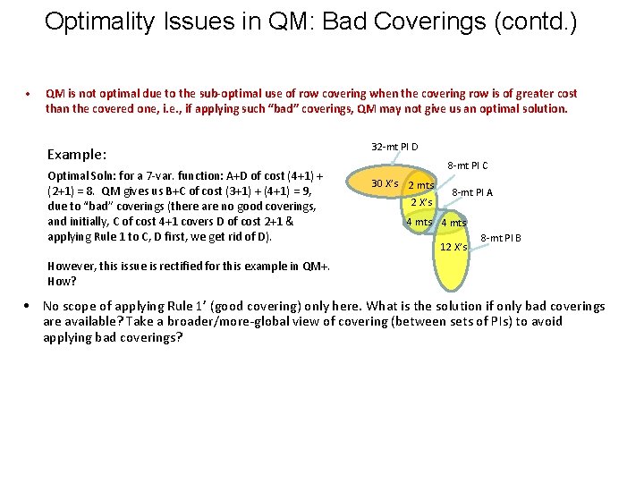
Optimality Issues in QM: Bad Coverings (contd. ) • QM is not optimal due to the sub-optimal use of row covering when the covering row is of greater cost than the covered one, i. e. , if applying such “bad” coverings, QM may not give us an optimal solution. Example: Optimal Soln: for a 7 -var. function: A+D of cost (4+1) + (2+1) = 8. QM gives us B+C of cost (3+1) + (4+1) = 9, due to “bad” coverings (there are no good coverings, and initially, C of cost 4+1 covers D of cost 2+1 & applying Rule 1 to C, D first, we get rid of D). 32 -mt PI D 8 -mt PI C 30 X’s 2 mts 2 X’s 8 -mt PI A 4 mts 12 X’s 8 -mt PI B However, this issue is rectified for this example in QM+. How? • No scope of applying Rule 1’ (good covering) only here. What is the solution if only bad coverings are available? Take a broader/more-global view of covering (between sets of PIs) to avoid applying bad coverings?

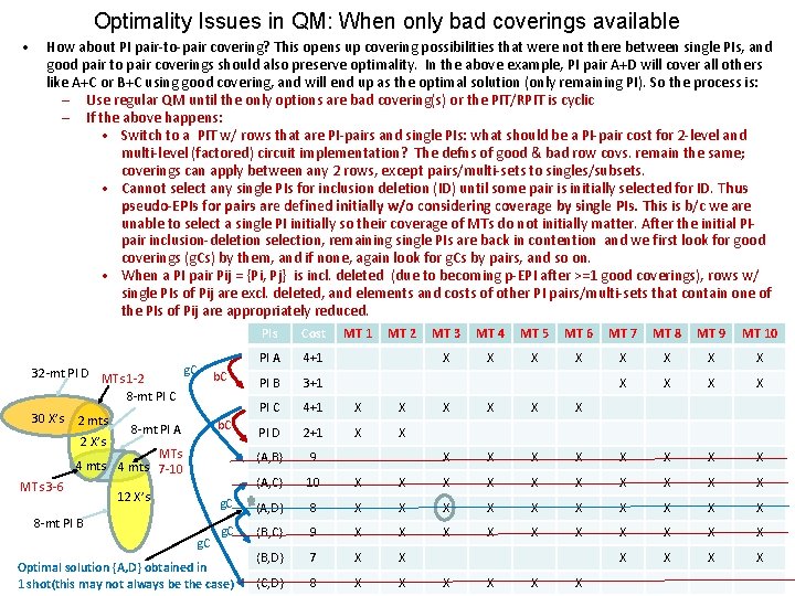
Optimality Issues in QM: When only bad coverings available • How about PI pair-to-pair covering? This opens up covering possibilities that were not there between single PIs, and good pair to pair coverings should also preserve optimality. In the above example, PI pair A+D will cover all others like A+C or B+C using good covering, and will end up as the optimal solution (only remaining PI). So the process is: ‒ Use regular QM until the only options are bad covering(s) or the PIT/RPIT is cyclic ‒ If the above happens: • Switch to a PIT w/ rows that are PI-pairs and single PIs: what should be a PI-pair cost for 2 -level and multi-level (factored) circuit implementation? The defns of good & bad row covs. remain the same; coverings can apply between any 2 rows, except pairs/multi-sets to singles/subsets. • Cannot select any single PIs for inclusion deletion (ID) until some pair is initially selected for ID. Thus pseudo-EPIs for pairs are defined initially w/o considering coverage by single PIs. This is b/c we are unable to select a single PI initially so their coverage of MTs do not initially matter. After the initial PIpair inclusion-deletion selection, remaining single PIs are back in contention and we first look for good coverings (g. Cs) by them, and if none, again look for g. Cs by pairs, and so on. • When a PI pair Pij = {Pi, Pj} is incl. deleted (due to becoming p-EPI after >=1 good coverings), rows w/ single PIs of Pij are excl. deleted, and elements and costs of other PI pairs/multi-sets that contain one of the PIs of Pij are appropriately reduced. 32 -mt PI D MTs 1 -2 8 -mt PI C 30 X’s 2 mts 2 X’s g. C PIs Cost PI A 4+1 PI B 3+1 PI C 4+1 X X PI D 2+1 X X {A, B} 9 {A, C} 10 X g. C {A, D} 8 g. C {B, C} b. C 8 -mt PI A MTs 4 mts 7 -10 MTs 3 -6 12 X’s 8 -mt PI B g. C Optimal solution {A, D} obtained in 1 shot(this may not always be the case) MT 1 MT 2 MT 3 MT 4 MT 5 MT 6 MT 7 MT 8 MT 9 MT 10 X X X X X X X X X X X 9 X X X X X {B, D} 7 X X X {C, D} 8 X X X

Optimality Issues in QM: When only bad coverings available (contd) • However, a similar problem comes up if the only pair-to-pair coverings are bad ones or there are none (what to do then? ). So this approach can mitigate the sub-optimality of single PI bad coverings (or no coverings in a cyclic PIT) due to good pair-to-pair coverings that open up, but not always. • We can take the concept further to triple-PI sets, then quadruple-PI sets, etc. , but in the extreme this approach “degenerates” into Petrick’s algorithm, which essentially considers all possible multi-PI sets that cover all MTs, and thus cover each other (and we only apply good coverings in this case, which are guaranteed to exist as we are considering all multi-PI sets—the optimal one good covers all others!).

Optimality Issues in QM (contd. ): Proof of optimality of “good” covering • Theorem: If row PIj covers row PIk in a PIT/RPIT and cost(PIj) <= cost(PIk) (this is the socalled “good” covering), then if PIk is exclusion deleted from the RPIT (i. e. , PIk will not be included in the final SOP expression f), then this leads to a cost of the final SOP expression f that is <= the cost of f if PIk is not exclusion deleted (i. e. , PIk is included in the final expr. ) • Proof: Two cases: 1. Case 1: PIk is not in any optimal solution. Clearly, in this case, optimality of the final solution will not be affected by exclusion deleting PIk 2. Case 2: PIk is in some optimal solution S. a) If PIj is also in the same solution, then we can reduce its cost by deleting PIk from S without affecting MT coverage in S (since PIj covers all the MTs of PIk not covered by “previously”-chosen EPIs or p-EPIs). Thus we reach a contradiction that S is an optimal solution. b) If PIj is not in S, we can replace PIk by PIj in S without affecting MT coverage in S, and reduce the cost of S or keep it the same (if cost(PIj) = cost(PIk) ). In the latter case, we get another optimal solution S’ that does not contain Pik Thus either PIk is not in any optimal solution or if it is, then we can get another optimal solution (i. e. , one with the same cost) containing PIj instead of PIk. Hence optimality of the final solution will not be affected by exclusion deleting PIk QED

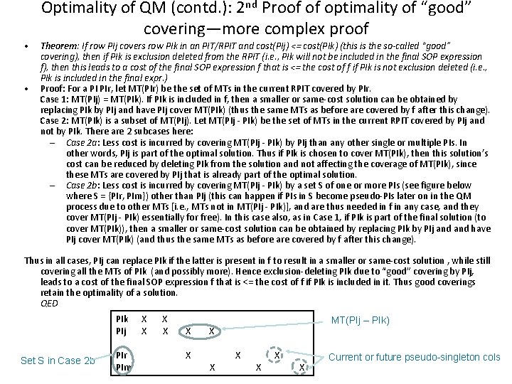
• • Optimality of QM (contd. ): 2 nd Proof of optimality of “good” covering—more complex proof Theorem: If row PIj covers row PIk in an PIT/RPIT and cost(PIj) <= cost(PIk) (this is the so-called “good” covering), then if PIk is exclusion deleted from the RPIT (i. e. , PIk will not be included in the final SOP expression f), then this leads to a cost of the final SOP expression f that is <= the cost of f if PIk is not exclusion deleted (i. e. , PIk is included in the final expr. ) Proof: For a PI PIr, let MT(PIr) be the set of MTs in the current RPIT covered by PIr. Case 1: MT(PIj) = MT(PIk). If PIk is included in f, then a smaller or same-cost solution can be obtained by replacing PIk by PIj and have PIj cover MT(PIk) (thus the same MTs as before are covered by f after this change). Case 2: MT(PIk) is a subset of MT(PIj). Let MT(PIj - PIk) be the set of MTs in the current RPIT covered by PIj and not by PIk. There are 2 subcases here: – Case 2 a: Less cost is incurred by covering MT(PIj - PIk) by PIj than any other single or multiple PIs. In other words, PIj is part of the optimal solution. Thus if PIk is chosen to cover MT(PIk), then this solution’s cost can be reduced by deleting PIk from the solution and not affecting the coverage of MT(PIk), since these MTs are covered by PIj that is already part of the optimal solution. – Case 2 b: Less cost is incurred by covering MT(PIj - PIk) by a set S of one or more PIs (see figure below where S = {PIr, PIm}) other than PIj (this can happen if PIs in S become pseudo-PIs later on in the QM process due to other MTs [i. e. , MTs not in MT(PIj - PIk)], and are thus needed in f in any case, and they cover MT(PIj - PIk) essentially for free). In this case also, as in Case 1, if PIk is part of the final solution (to cover MT(PIk)), then a smaller or same-cost solution can be obtained by replacing PIk by PIj and have PIj cover MT(PIk) (and thus the same MTs as before are covered by f after this change). Thus in all cases, PIj can replace PIk if the latter is present in f to result in a smaller or same-cost solution , while still covering all the MTs of PIk (and possibly more). Hence exclusion-deleting PIk due to “good” covering by PIj, leads to a cost of the final SOP expression f that is <= the cost of f if PIk is included in it. Thus good coverings retain the optimality of a solution. QED PIk PIj Set S in Case 2 b PIr PIm X X X MT(PIj – PIk) X X X Current or future pseudo-singleton cols