ECE 465 FSM State Minimization for Completely Specified

ECE 465 FSM State Minimization for Completely Specified Machines Shantanu Dutt Acknowledgement: Slides prepared by Huan Ren from Prof. Dutt’s Lecture Notes (some modifications made by Prof. Dutt)

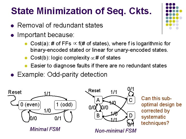
State Minimization of Seq. Ckts. l l Removal of redundant states Important because: l l Cost(a): # of FFs f(# of states), where f is logarithmic for binary-encoded stated or linear for unary-encoded states. Cost(b): logic complexity # of states Easier to diagnose faults if there are no redundant states Example: Odd-parity detection Reset 1/1 0 (even) 1 (odd) 1/0 0/1 Minimal FSM 1/1 A 0/0 B 1/0 1/1 0/1 C D 0/1 Non-minimal FSM Can this suboptimal design be corrected by systematic techniques?

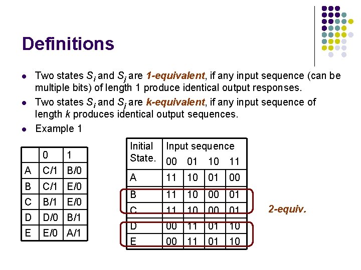
Definitions l l l Two states Si and Sj are 1 -equivalent, if any input sequence (can be multiple bits) of length 1 produce identical output responses. Two states Si and Sj are k-equivalent, if any input sequence of length k produces identical output sequences. Example 1 0 1 A C/1 B/0 B C/1 E/0 C B/1 E/0 D D/0 B/1 E E/0 A/1 Initial Input sequence State. 00 01 10 11 A 11 10 01 00 B 11 10 00 01 C 11 10 00 01 D 00 11 01 10 E 00 11 01 10 2 -equiv.

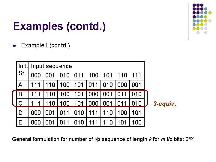
Examples (contd. ) l Example 1 (contd. ) Init. Input sequence St. 000 001 010 011 100 101 110 111 A 111 110 101 010 001 B 111 110 101 000 001 010 C 111 110 101 000 001 010 D 000 001 010 111 110 101 E 000 001 010 111 110 101 100 3 -equiv. General formulation for number of i/p sequence of length k for m i/p bits: 2 mk

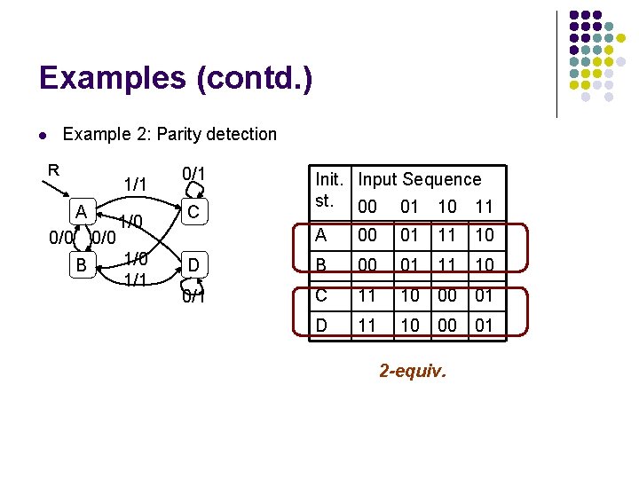
Examples (contd. ) Example 2: Parity detection l R 1/1 A 0/0 B 1/0 1/1 0/1 C Init. Input Sequence st. 00 01 10 11 A 00 01 11 10 D B 00 01 11 10 0/1 C 11 10 00 01 D 11 10 00 01 2 -equiv.

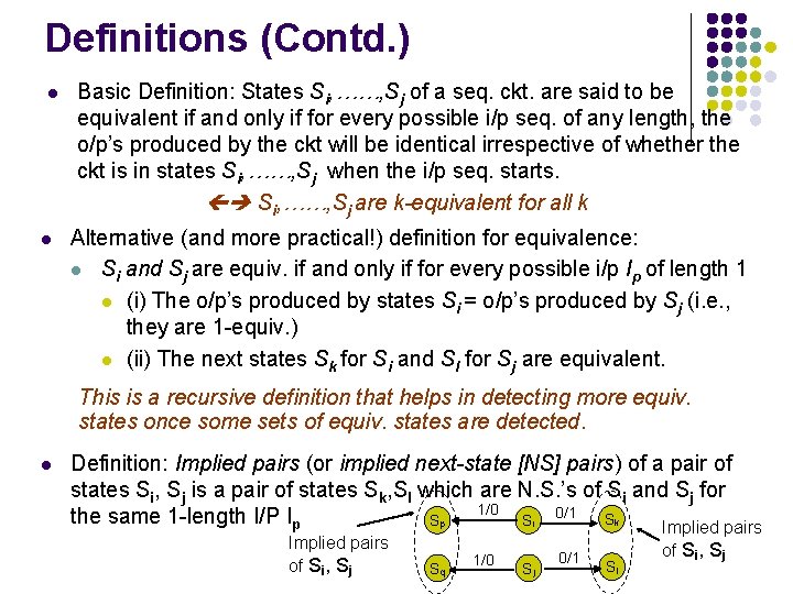
Definitions (Contd. ) l l Basic Definition: States Si, ……, Sj of a seq. ckt. are said to be equivalent if and only if for every possible i/p seq. of any length, the o/p’s produced by the ckt will be identical irrespective of whether the ckt is in states Si, ……, Sj when the i/p seq. starts. Si, ……, Sj are k-equivalent for all k Alternative (and more practical!) definition for equivalence: l Si and Sj are equiv. if and only if for every possible i/p Ip of length 1 l (i) The o/p’s produced by states Si = o/p’s produced by Sj (i. e. , they are 1 -equiv. ) l (ii) The next states Sk for Si and Sl for Sj are equivalent. This is a recursive definition that helps in detecting more equiv. states once some sets of equiv. states are detected. l Definition: Implied pairs (or implied next-state [NS] pairs) of a pair of states Si, Sj is a pair of states Sk, Sl which are N. S. ’s of Si and Sj for 1/0 the same 1 -length I/P Ip Sk Sp Si 0/1 Implied pairs of Si, Sj Sq 1/0 Sj 0/1 Sl of Si, Sj

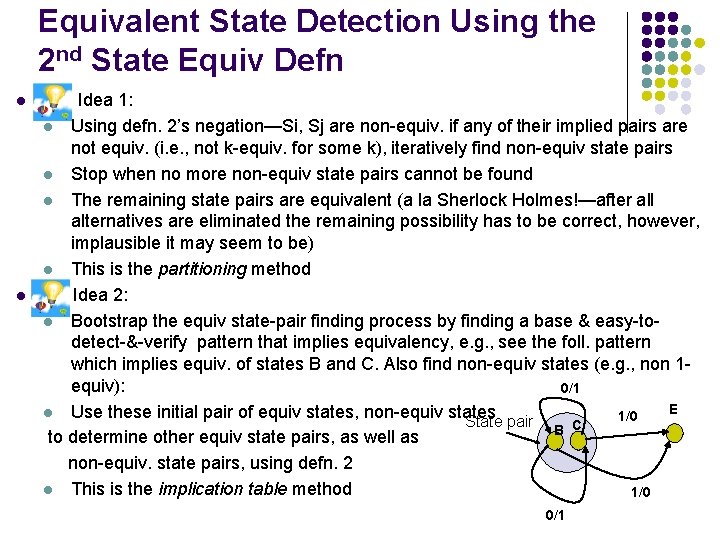
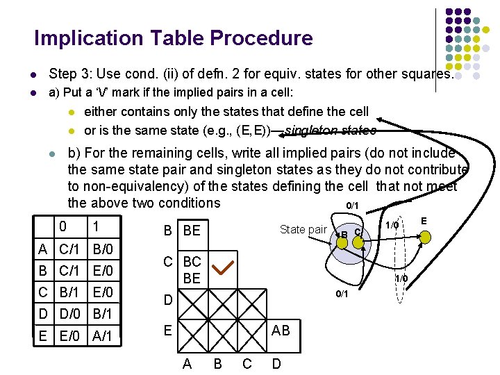
Equivalent State Detection Using the 2 nd State Equiv Defn l l Idea 1: l Using defn. 2’s negation—Si, Sj are non-equiv. if any of their implied pairs are not equiv. (i. e. , not k-equiv. for some k), iteratively find non-equiv state pairs l Stop when no more non-equiv state pairs cannot be found l The remaining state pairs are equivalent (a la Sherlock Holmes!—after all alternatives are eliminated the remaining possibility has to be correct, however, implausible it may seem to be) l This is the partitioning method Idea 2: l Bootstrap the equiv state-pair finding process by finding a base & easy-todetect-&-verify pattern that implies equivalency, e. g. , see the foll. pattern which implies equiv. of states B and C. Also find non-equiv states (e. g. , non 1 equiv): 0/1 E l Use these initial pair of equiv states, non-equiv states 1/0 State pair B C to determine other equiv state pairs, as well as non-equiv. state pairs, using defn. 2 l This is the implication table method 1/0 0/1

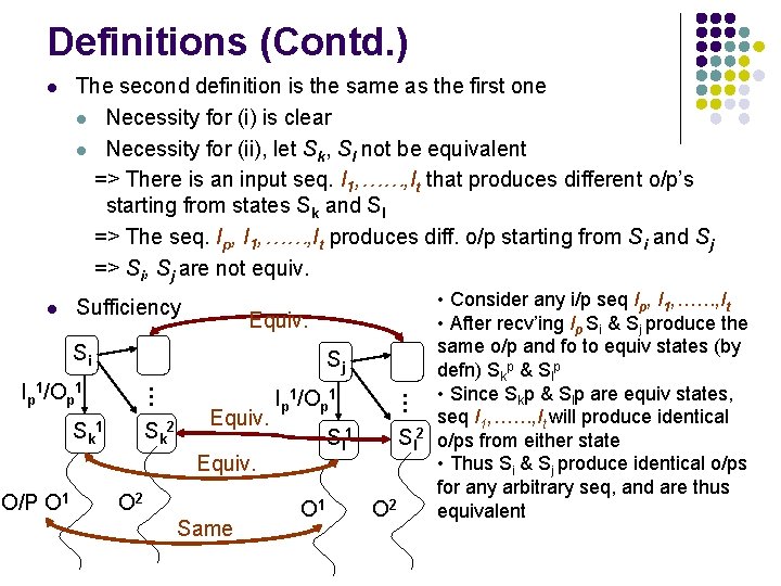
Definitions (Contd. ) l The second definition is the same as the first one l Necessity for (i) is clear l Necessity for (ii), let Sk, Sl not be equivalent => There is an input seq. I 1, ……, It that produces different o/p’s starting from states Sk and Sl => The seq. Ip, I 1, ……, It produces diff. o/p starting from Si and Sj => Si, Sj are not equiv. l Sufficiency Equiv. Si Sj Sk 1 Sk 2 Equiv. Ip 1/Op 1 Sl 1 Equiv. O/P O 1 O 2 Same … … Ip 1/Op 1 O 1 Sl 2 O 2 • Consider any i/p seq Ip, I 1, ……, It • After recv’ing Ip Si & Sj produce the same o/p and fo to equiv states (by defn) Skp & Slp • Since Skp & Slp are equiv states, seq I 1, ……, It will produce identical o/ps from either state • Thus Si & Sj produce identical o/ps for any arbitrary seq, and are thus equivalent

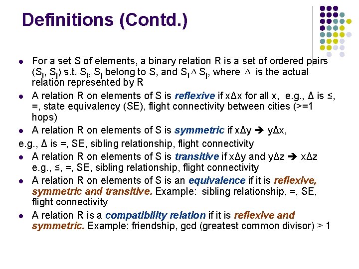
Definitions (Contd. ) For a set S of elements, a binary relation R is a set of ordered pairs (Si, Sj) s. t. Si, Sj belong to S, and SiΔSj, where Δ is the actual relation represented by R l A relation R on elements of S is reflexive if xΔx for all x, e. g. , Δ is ≤, =, state equivalency (SE), flight connectivity between cities (>=1 hops) l A relation R on elements of S is symmetric if xΔy yΔx, e. g. , Δ is =, SE, sibling relationship, flight connectivity l A relation R on elements of S is transitive if xΔy and yΔz xΔz e. g. , ≤, =, SE, sibling relationship, flight connectivity l A relation R on elements of S is an equivalence if it is reflexive, symmetric and transitive. Example: sibling relationship, =, SE, flight connectivity l A relation R is a compatibility relation if it is reflexive and symmetric. Example: friendship, gcd (greatest common divisor) > 1 l

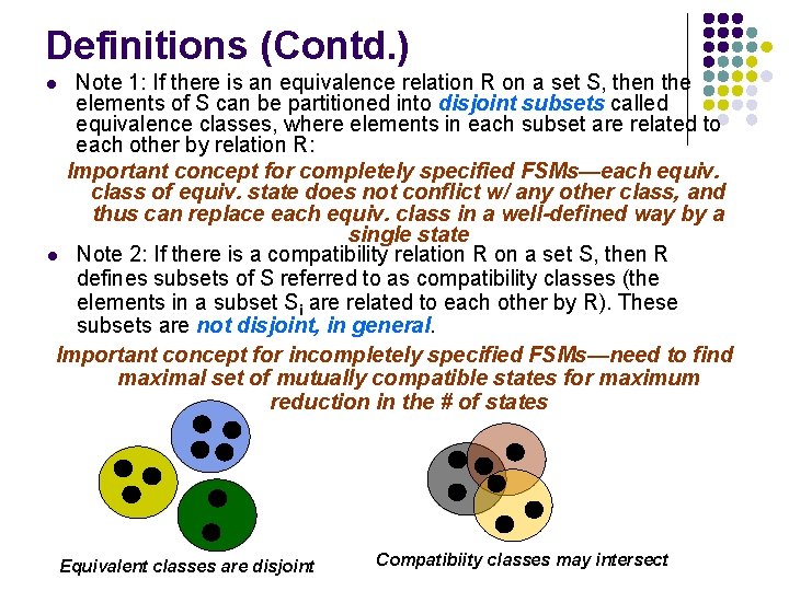
Definitions (Contd. ) Note 1: If there is an equivalence relation R on a set S, then the elements of S can be partitioned into disjoint subsets called equivalence classes, where elements in each subset are related to each other by relation R: Important concept for completely specified FSMs—each equiv. class of equiv. state does not conflict w/ any other class, and thus can replace each equiv. class in a well-defined way by a single state l Note 2: If there is a compatibility relation R on a set S, then R defines subsets of S referred to as compatibility classes (the elements in a subset Si are related to each other by R). These subsets are not disjoint, in general. Important concept for incompletely specified FSMs—need to find maximal set of mutually compatible states for maximum reduction in the # of states l Equivalent classes are disjoint Compatibiity classes may intersect

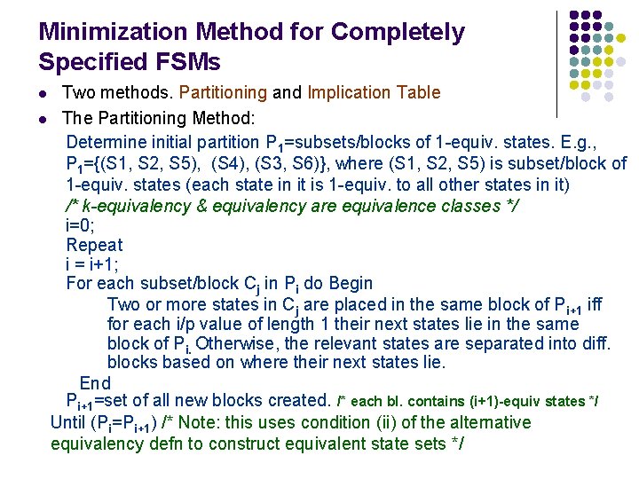
Minimization Method for Completely Specified FSMs Two methods. Partitioning and Implication Table l The Partitioning Method: Determine initial partition P 1=subsets/blocks of 1 -equiv. states. E. g. , P 1={(S 1, S 2, S 5), (S 4), (S 3, S 6)}, where (S 1, S 2, S 5) is subset/block of 1 -equiv. states (each state in it is 1 -equiv. to all other states in it) /* k-equivalency & equivalency are equivalence classes */ i=0; Repeat i = i+1; For each subset/block Cj in Pi do Begin Two or more states in Cj are placed in the same block of Pi+1 iff for each i/p value of length 1 their next states lie in the same block of Pi. Otherwise, the relevant states are separated into diff. blocks based on where their next states lie. End Pi+1=set of all new blocks created. /* each bl. contains (i+1)-equiv states */ Until (Pi=Pi+1) /* Note: this uses condition (ii) of the alternative equivalency defn to construct equivalent state sets */ l

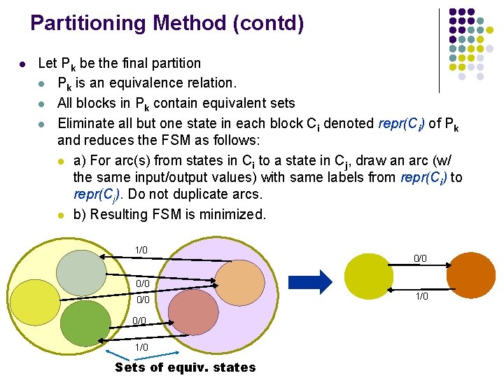
Partitioning Method (contd) l Let Pk be the final partition l Pk is an equivalence relation. l All blocks in Pk contain equivalent sets l Eliminate all but one state in each block Ci denoted repr(Ci) of Pk and reduces the FSM as follows: l a) For arc(s) from states in Ci to a state in Cj, draw an arc (w/ the same input/output values) with same labels from repr(Ci) to repr(Cj). Do not duplicate arcs. l b) Resulting FSM is minimized. 1/0 0/0 0/0 1/0 Sets of equiv. states 1/0

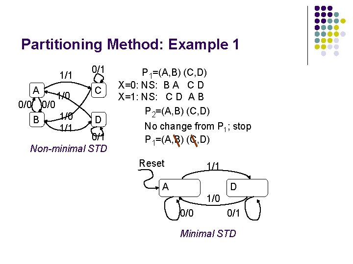
Partitioning Method: Example 1 1/1 A 0/0 B 1/0 1/1 0/1 C D 0/1 Non-minimal STD P 1=(A, B) (C, D) X=0: NS: B A C D X=1: NS: C D A B P 2=(A, B) (C, D) No change from P 1; stop P 1=(A, B) (C, D) Reset 1/1 A D 1/0 0/1 Minimal STD

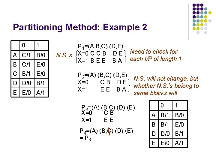
Partitioning Method: Example 2 0 1 A C/1 B/0 B C/1 E/0 C B/1 E/0 D D/0 B/1 E E/0 A/1 P 1=(A, B, C) (D, E) N. S. ’s X=0 C C B D E X=1 B E E B A Need to check for each I/P of length 1 P 2=(A) (B, C) (D, E) X=0 CB DE X=1 EE BA N. S. will not change, but whether N. S. ’s belong to same blocks will 0 1 P 3=(A) (B, C) (D) (E) X=0 CB X=1 EE A B/1 B/0 P 4=(A) (B, C) (D) (E) = P 3 D D/0 B/1 B B/1 E/0 E E/0 A/1

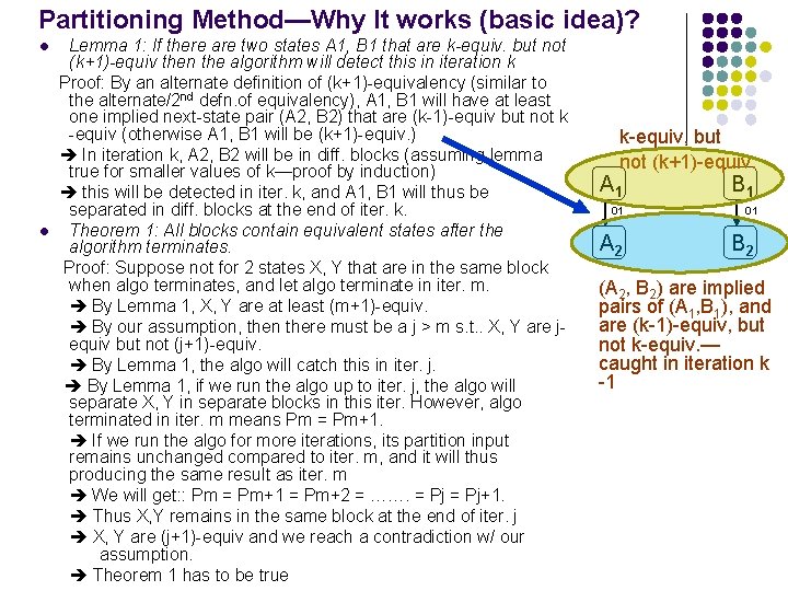
Partitioning Method—Why It works (basic idea)? l l Lemma 1: If there are two states A 1, B 1 that are k-equiv. but not (k+1)-equiv then the algorithm will detect this in iteration k Proof: By an alternate definition of (k+1)-equivalency (similar to the alternate/2 nd defn. of equivalency), A 1, B 1 will have at least one implied next-state pair (A 2, B 2) that are (k-1)-equiv but not k -equiv (otherwise A 1, B 1 will be (k+1)-equiv. ) In iteration k, A 2, B 2 will be in diff. blocks (assuming lemma true for smaller values of k—proof by induction) this will be detected in iter. k, and A 1, B 1 will thus be separated in diff. blocks at the end of iter. k. Theorem 1: All blocks contain equivalent states after the algorithm terminates. Proof: Suppose not for 2 states X, Y that are in the same block when algo terminates, and let algo terminate in iter. m. By Lemma 1, X, Y are at least (m+1)-equiv. By our assumption, then there must be a j > m s. t. . X, Y are jequiv but not (j+1)-equiv. By Lemma 1, the algo will catch this in iter. j. By Lemma 1, if we run the algo up to iter. j, the algo will separate X, Y in separate blocks in this iter. However, algo terminated in iter. m means Pm = Pm+1. If we run the algo for more iterations, its partition input remains unchanged compared to iter. m, and it will thus producing the same result as iter. m We will get: : Pm = Pm+1 = Pm+2 = ……. = Pj+1. Thus X, Y remains in the same block at the end of iter. j X, Y are (j+1)-equiv and we reach a contradiction w/ our assumption. Theorem 1 has to be true k-equiv, but not (k+1)-equiv. A 1 01 A 2 B 1 01 B 2 (A 2, B 2) are implied pairs of (A 1, B 1), and are (k-1)-equiv, but not k-equiv. — caught in iteration k -1

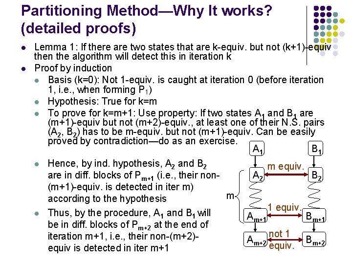
Partitioning Method—Why It works? (detailed proofs) l l Lemma 1: If there are two states that are k-equiv. but not (k+1)-equiv then the algorithm will detect this in iteration k Proof by induction l Basis (k=0): Not 1 -equiv. is caught at iteration 0 (before iteration 1, i. e. , when forming P 1) l Hypothesis: True for k=m l To prove for k=m+1: Use property: If two states A 1 and B 1 are (m+1)-equiv but not (m+2)-equiv. , at least one of their N. S. pairs (A 2, B 2) has to be m-equiv. but not (m+1)-equiv. Can be easily proved by contradiction—do as an exercise. A 1 B 1 l Hence, by ind. hypothesis, A 2 and B 2 m equiv. are in diff. blocks of Pm+1 (i. e. , their non. A 2 B 2 (m+1)-equiv. is detected in iter m) m according to the hypothesis 1 equiv. l Thus, by the procedure, A 1 and B 1 will Am+1 Bm+1 be in diff. blocks of Pm+2 at the end of not 1 iteration m+1, i. e. , their non-(m+2)Am+2 Bm+2 equiv is detected in iter m+1

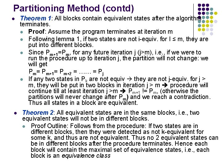
Partitioning Method (contd) l l Theorem 1: All blocks contain equivalent states after the algorithm terminates. l Proof: Assume the program terminates at iteration m l Following lemma 1, if two states are not i-equiv. for I ≤ m, they are put into different blocks. l Since Pm+1=Pm, for any future iteration j (j>m), i. e. , if we were to run the procedure up to iteration j, the partition will not change: we will get Pm= Pm+1= Pm+2 = …… = Pj l If any two states in Pk are not equiv they are not j-equiv. for j > m, they will be put in two blocks in iteration j > m procedure will continue till at least iteration j >m Pm+1 != Pm, (otherwise the partitions will never change after Pm) and we reach a contradiction. Thus all states in a block are equivalent. Theorem 2: All equivalent states are in the same blocks, i. e. , two equivalent states will not be in different blocks. l Proof Outline: Follows from the procedure: If two states are in different blocks, then they were detected as not k-equivalent for some k, and thus are not equivalent. Thus no 2 equivalent states can be in different blocks after the procedure terminates. Hence each block will contain the maximal set of equivalence states, i. e. , each block is an equivalence class

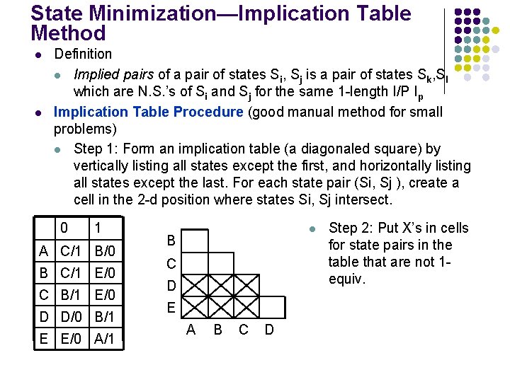
State Minimization—Implication Table Method l l Definition l Implied pairs of a pair of states Si, Sj is a pair of states Sk, Sl which are N. S. ’s of Si and Sj for the same 1 -length I/P Ip Implication Table Procedure (good manual method for small problems) l Step 1: Form an implication table (a diagonaled square) by vertically listing all states except the first, and horizontally listing all states except the last. For each state pair (Si, Sj ), create a cell in the 2 -d position where states Si, Sj intersect. 0 1 A C/1 B/0 B C/1 E/0 C B/1 E/0 D D/0 B/1 E E/0 A/1 l B C D E A B C D Step 2: Put X’s in cells for state pairs in the table that are not 1 equiv.

Implication Table Procedure l Step 3: Use cond. (ii) of defn. 2 for equiv. states for other squares. l a) Put a ‘/’ mark if the implied pairs in a cell: l l either contains only the states that define the cell or is the same state (e. g. , (E, E))—singleton states b) For the remaining cells, write all implied pairs (do not include the same state pair and singleton states as they do not contribute to non-equivalency) of the states defining the cell that not meet the above two conditions 0/1 l 0 1 A C/1 B/0 B C/1 E/0 C B/1 E/0 D D/0 B/1 E E/0 A/1 B BE State pair B C C BC BE 1/0 0/1 D E AB A 1/0 B C D E

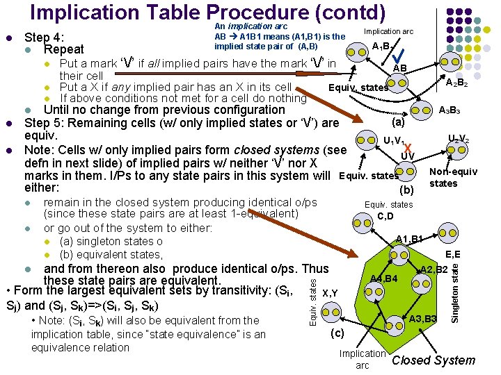
Implication Table Procedure (contd) Step 4: l Repeat l l l Implication arc A 1 B 1 Put a mark ‘/’ if all implied pairs have the mark ‘/’ in AB their cell Equiv. states Put a X if any implied pair has an X in its cell If above conditions not met for a cell do nothing A 2 B 2 Until no change from previous configuration (a) Step 5: Remaining cells (w/ only implied states or ‘/’) are equiv. U 1 V 1 X Note: Cells w/ only implied pairs form closed systems (see UV defn in next slide) of implied pairs w/ neither ‘/’ nor X marks in them. I/Ps to any state pairs in this system will Equiv. states either: (b) A 3 B 3 l l l remain in the closed system producing identical o/ps (since these state pairs are at least 1 -equivalent) or go out of the system to either: l l Non-equiv states Equiv. states C, D A 1, B 1 (a) singleton states o (b) equivalent states, E, E and from thereon also produce identical o/ps. Thus these state pairs are equivalent. • Form the largest equivalent sets by transitivity: (Si, X, Y Sj) and (Sj, Sk)=>(Si, Sj, Sk) • Note: (Si, Sk) will also be equivalent from the l A 4, B 4 Equiv. states implication table, since “state equivalence” is an equivalence relation U 2 V 2 A 2, B 2 A 3, B 3 Singleton state l An implication arc AB A 1 B 1 means (A 1, B 1) is the implied state pair of (A, B) (c) Implication arc Closed System

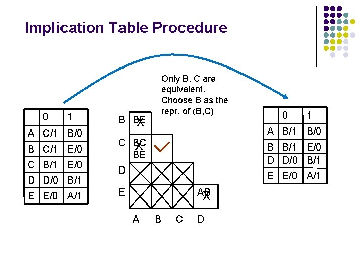
Implication Table Procedure 0 1 A C/1 B/0 B C/1 E/0 C B/1 E/0 D D/0 B/1 E E/0 A/1 B BE X Only B, C are equivalent. Choose B as the repr. of (B, C) 0 1 A B/1 B/0 C BC X BE B B/1 E/0 D D/0 B/1 D E E/0 A/1 E AB X A B C D

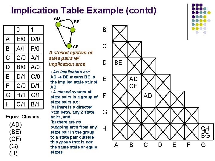
Implication Table Example (contd) AD 0 B 1 A E/0 D/0 B A/1 F/0 C C/0 A/1 D B/0 A/0 E D/1 C/0 F C/0 D/1 G H/1 G/1 H C/1 B/1 Equiv. Classes: (AD) (BE) (CF) (G) (H) BE CF A closed system of state pairs w/ implication arcs • An implication arc AD BE means BE is the implied state pair of AD • A closed system of state pairs is a group of state pairs s. t. : (a) there is a directed path betw. any 2 state pairs, and (b) there are no outgoing arcs from any state pair in the group to a state pair outside this group that is not the same state or equiv states C D BE E AD CF F AD G H CH X BG A B C D E F G

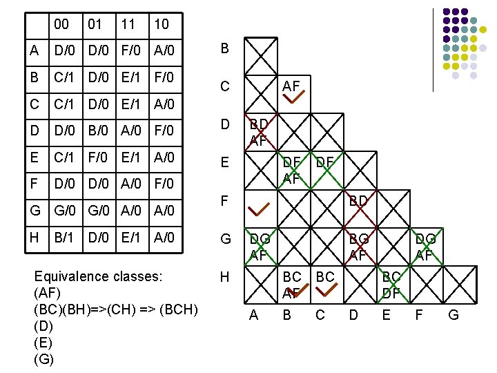
00 01 11 10 B A D/0 F/0 A/0 B C/1 D/0 E/1 F/0 C C/1 D/0 E/1 A/0 D D/0 B/0 A/0 F/0 D E C/1 F/0 E/1 A/0 E F D/0 A/0 F/0 G G/0 A/0 H C AF BD AF DF F B/1 D/0 E/1 A/0 G Equivalence classes: (AF) (BC)(BH)=>(CH) => (BCH) (D) (E) (G) H BD DG AF A BG AF BC B C DG AF BC DF D E F G

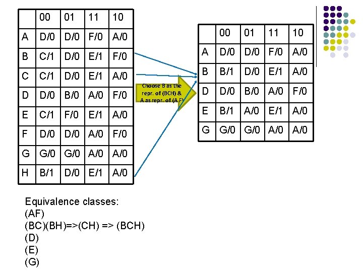
00 01 11 10 A D/0 F/0 A/0 B C/1 D/0 E/1 F/0 A D/0 F/0 A/0 C C/1 D/0 E/1 A/0 B B/1 D/0 E/1 A/0 D D/0 B/0 A/0 F/0 B/1 A/0 E/1 A/0 Choose B as the repr. of (BCH) & A as repr. of (A F) D D/0 B/0 A/0 F/0 E C/1 F/0 E/1 A/0 E F D/0 A/0 F/0 G G/0 G/0 A/0 A/0 H B/1 D/0 E/1 A/0 Equivalence classes: (AF) (BC)(BH)=>(CH) => (BCH) (D) (E) (G)

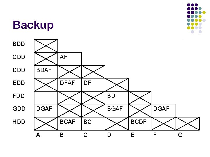
Backup BDD CDD DDD AF BDAF EDD DFAF DF FDD GDD BD DGAF HDD A BGAF BC B C DGAF BCDF D E F G