Production Costs ECO 61 Udayan Roy Fall 2008

Production Costs ECO 61 Udayan Roy Fall 2008

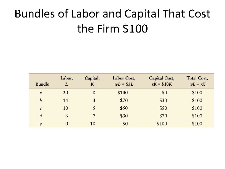
Bundles of Labor and Capital That Cost the Firm $100

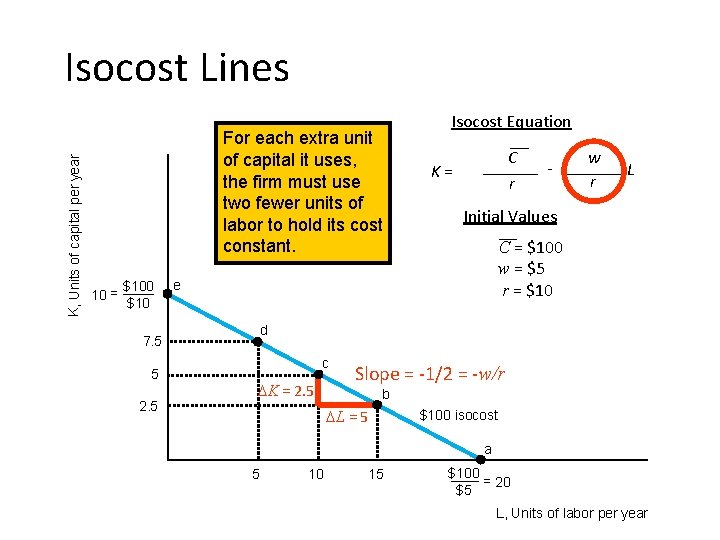
K, Units of capital per year Isocost Lines For each extra unit of capital it uses, the firm must use two fewer units of labor to hold its cost constant. 10 = $100 $10 2. 5 C r K= - w r L Initial Values C = $100 w = $5 r = $10 e d 7. 5 5 Isocost Equation c DK = 2. 5 Slope = -1/2 = -w/r b DL = 5 $100 isocost a 5 10 15 $100 = 20 $5 L, Units of labor per year

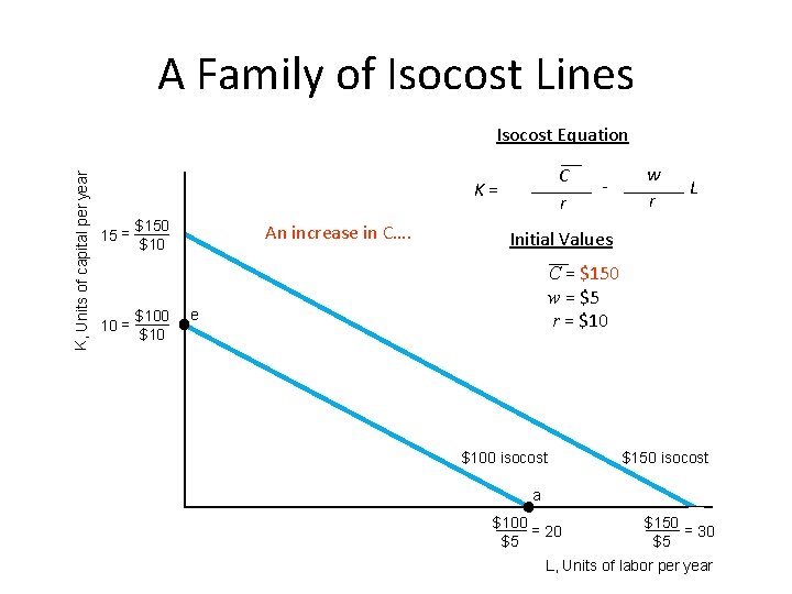
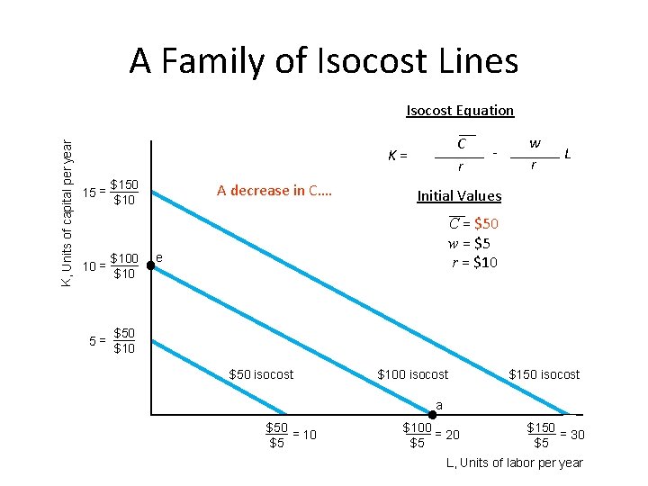
A Family of Isocost Lines K, Units of capital per year Isocost Equation C r K= 15 = 10 = $150 $100 $10 An increase in C…. - w r L Initial Values C = $150 w = $5 r = $10 e $100 isocost $150 isocost a $100 = 20 $5 $150 = 30 $5 L, Units of labor per year

A Family of Isocost Lines K, Units of capital per year Isocost Equation C r K= 15 = $150 $10 10 = $100 $10 5= $50 $10 A decrease in C…. - w r L Initial Values C = $50 w = $5 r = $10 e $50 isocost $100 isocost $150 isocost a $50 = 10 $5 $100 = 20 $5 $150 = 30 $5 L, Units of labor per year

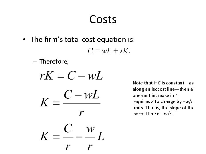
Costs • The firm’s total cost equation is: C = w. L + r. K. – Therefore, Note that if C is constant—as along an isocost line—then a one-unit increase in L requires K to change by –w/r units. That is, the slope of the isocost line is –w/r.

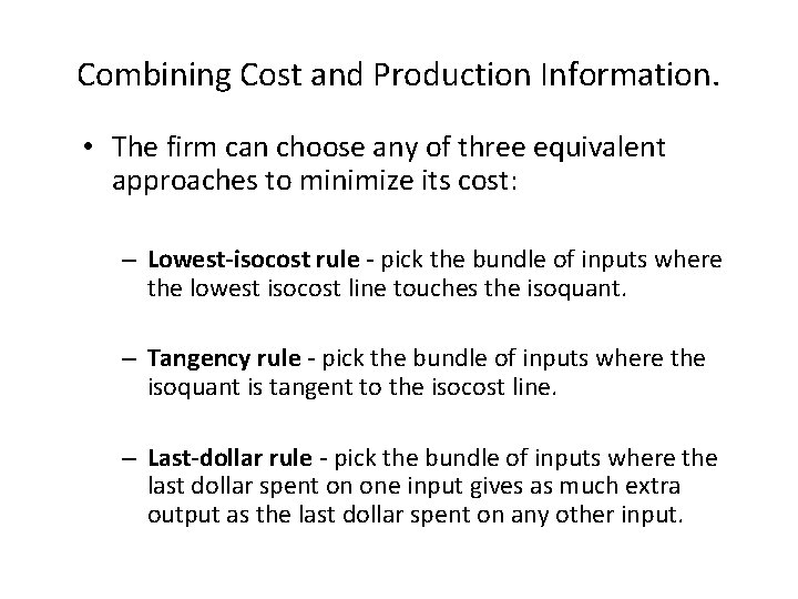
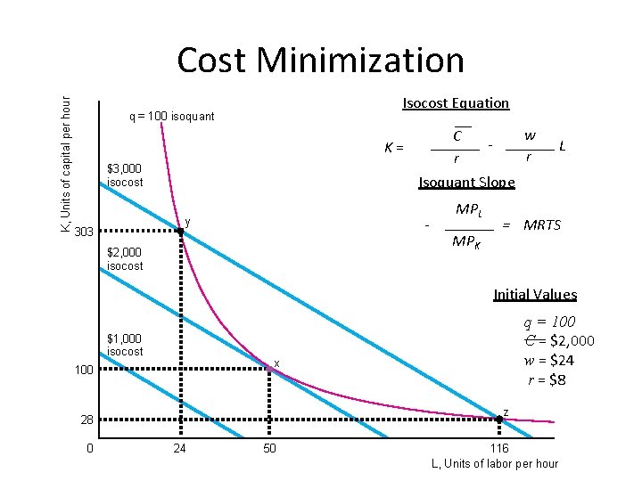
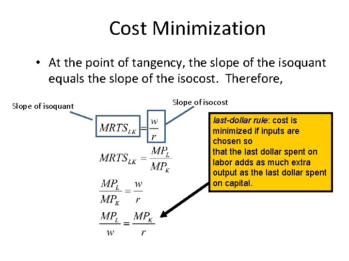
Combining Cost and Production Information. • The firm can choose any of three equivalent approaches to minimize its cost: – Lowest-isocost rule - pick the bundle of inputs where the lowest isocost line touches the isoquant. – Tangency rule - pick the bundle of inputs where the isoquant is tangent to the isocost line. – Last-dollar rule - pick the bundle of inputs where the last dollar spent on one input gives as much extra output as the last dollar spent on any other input.

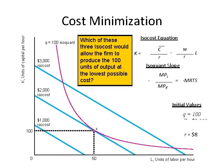
K, Units of capital per hour Cost Minimization q = 100 isoquant $3, 000 isocost Which of these three Isocost would allow the firm to produce the 100 units of output at the lowest possible cost? $2, 000 isocost Isocost Equation w C K= r r Isoquant Slope - MPL MPK L = -MRTS Initial Values $1, 000 isocost 100 0 x 50 q = 100 C = $2, 000 w = $24 r = $8 L, Units of labor per hour

K, Units of capital per hour Cost Minimization Isocost Equation q = 100 isoquant K= $3, 000 isocost y 303 w C r r Isoquant Slope - $2, 000 isocost MPL MPK L = MRTS Initial Values $1, 000 isocost x 100 z 28 0 q = 100 C = $2, 000 w = $24 r = $8 24 50 116 L, Units of labor per hour

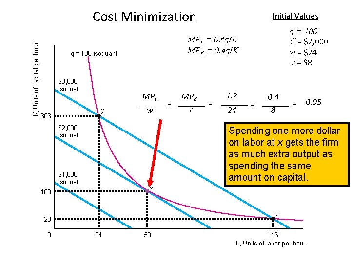
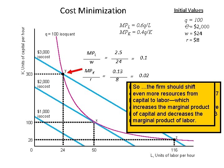
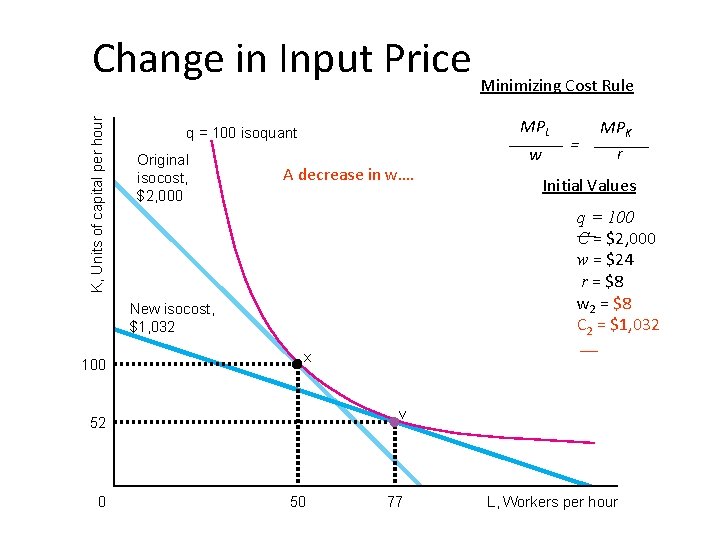
Cost Minimization • At the point of tangency, the slope of the isoquant equals the slope of the isocost. Therefore, Slope of isoquant Slope of isocost last-dollar rule: cost is minimized if inputs are chosen so that the last dollar spent on labor adds as much extra output as the last dollar spent on capital.

K, Units of capital per hour Cost Minimization MPL y 303 w $2, 000 isocost = MPK r = 1. 2 24 = 0. 4 8 = 0. 05 Spending one more dollar on labor at x gets the firm as much extra output as spending the same amount on capital. $1, 000 isocost x 100 z 28 0 q = 100 C = $2, 000 w = $24 r = $8 MPL = 0. 6 q/L MPK = 0. 4 q/K q = 100 isoquant $3, 000 isocost Initial Values 24 50 116 L, Units of labor per hour

K, Units of capital per hour Cost Minimization MPL w y 303 $2, 000 isocost $1, 000 isocost MPK r 2. 5 24 0. 13 8 = 0. 1 = 0. 02 firm should shiftfrom if So the…the firm shifts one dollar even more resources fromby 0. 017 capital to labor, output falls capital to labor—which because there is less capital but increases the by marginal product also increases 0. 1 because there capital and isof more labor fordecreases a net gainthe of 0. 083 marginal product of labor. more output at the same cost…. z 28 0 = = x 100 q = 100 C = $2, 000 w = $24 r = $8 MPL = 0. 6 q/L MPK = 0. 4 q/K q = 100 isoquant $3, 000 isocost Initial Values 24 50 116 L, Units of labor per hour

K, Units of capital per hour Change in Input Price Minimizing Cost Rule MPL q = 100 isoquant Original isocost, $2, 000 A decrease in w…. Initial Values x v 52 0 = q = 100 C = $2, 000 w = $24 r = $8 w 2 = $8 C 2 = $1, 032 New isocost, $1, 032 100 w MPK r 50 77 L, Workers per hour

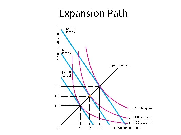
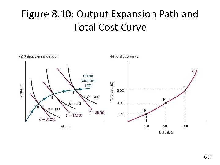
How Long-Run Cost Varies with Output • expansion path - the cost-minimizing combination of labor and capital for each output level

K, Units of capital per hour Expansion Path $4, 000 isocost $3, 000 isocost Expansion path $2, 000 isocost z 200 y 150 x 100 q = 300 Isoquant q = 200 Isoquant q = 100 Isoquant 0 50 75 100 L, Workers per hour

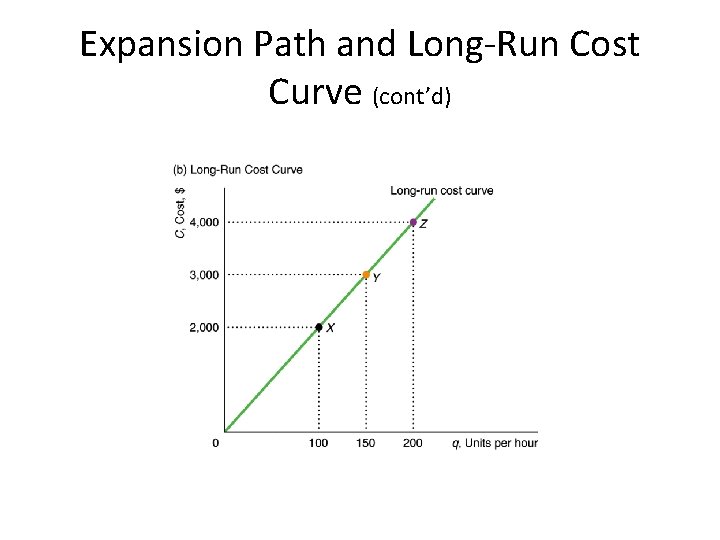
Expansion Path and Long-Run Cost Curve (cont’d)

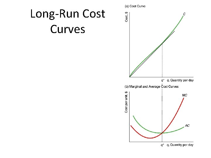
Long-Run Cost Curves

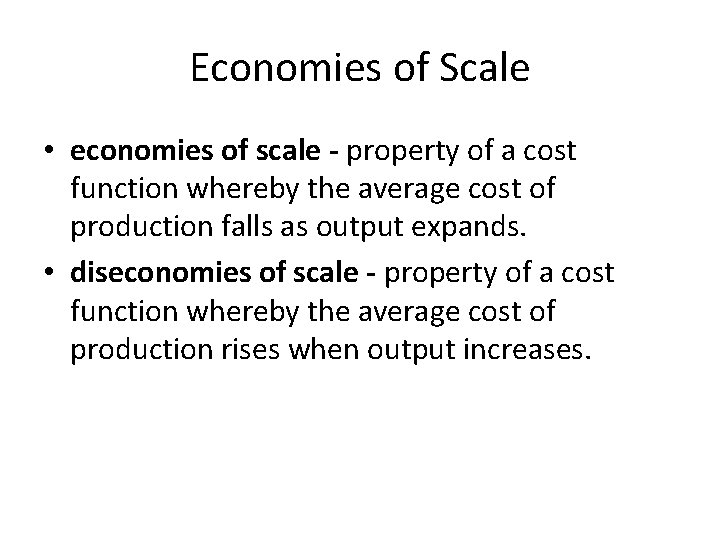
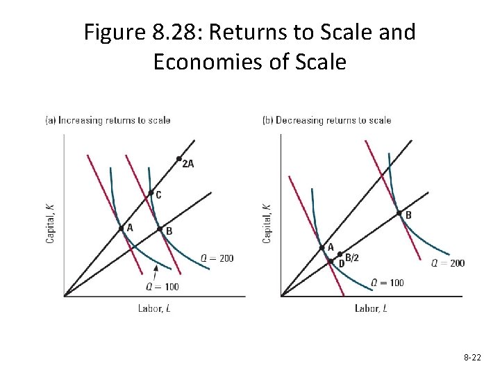
Economies of Scale • economies of scale - property of a cost function whereby the average cost of production falls as output expands. • diseconomies of scale - property of a cost function whereby the average cost of production rises when output increases.

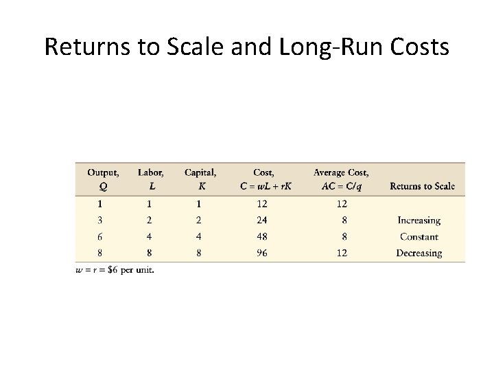
Returns to Scale and Long-Run Costs

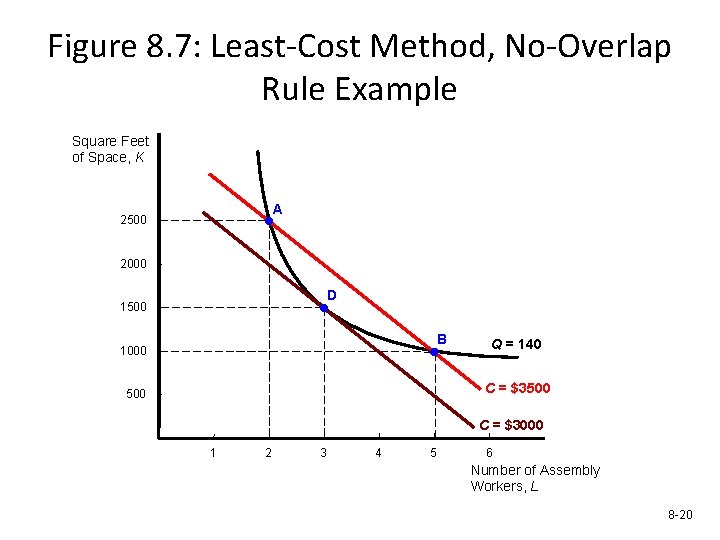
Figure 8. 7: Least-Cost Method, No-Overlap Rule Example Square Feet of Space, K A 2500 2000 D 1500 B 1000 Q = 140 C = $3500 C = $3000 1 2 3 4 5 6 Number of Assembly Workers, L 8 -20

Figure 8. 10: Output Expansion Path and Total Cost Curve 8 -21

Figure 8. 28: Returns to Scale and Economies of Scale 8 -22