Chapter 21 Cost Minimization Key Concept Cost minimization

• Chapter 21 Cost Minimization • Key Concept: Cost minimization implies isoquant and isocost are tangent to each other MP 1(x 1*, x 2*)/MP 2(x 1*, x 2*) = w 1/w 2 • LR total cost curve is the lower envelope of the SR total cost curves.

• Chapter 21 Cost Minimization • Break max to • 1) cost min for every y • 2) choose the optimal y* (to max ).

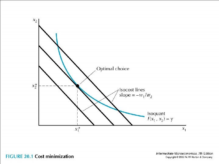
• The cost minimization problems is: minx 1, x 2 w 1 x 1+w 2 x 2 st. f(x 1, x 2)=y • Denote the solution the cost function c(w 1, w 2, y). • It measures the minimal costs of producing y units of outputs when the input prices are (w 1, w 2).

• On the x 1 -x 2 plane, we can draw the family of isocost curves. • A typical one takes the form of w 1 x 1+w 2 x 2=k, having the slope of -w 1/w 2.

• At optimum, the usual tangency condition says that • MRTS 1, 2(x 1*, x 2*) =∆x 2/∆x 1 =-MP 1(x 1*, x 2*)/MP 2(x 1*, x 2*) = -w 1/w 2.

• MRTS 1, 2(x 1*, x 2*) =∆x 2/∆x 1 =-MP 1(x 1*, x 2*)/MP 2(x 1*, x 2*) = -w 1/w 2. • Rearranging to get MP 1(x 1*, x 2*)/w 1= MP 2(x 1*, x 2*)/w 2 an extra dollar spent on recruiting factor 1 or 2 would yield the same extra amount of outputs.

• The optimal choices of inputs are denoted as x 1(w 1, w 2, y) and x 2(w 1, w 2, y). • These are called the conditional factor demands or derived factor demands. • These are hypothetical constructs, usually not observed.

• Some examples. • f(x 1, x 2)=min{x 1, x 2}: c(w 1, w 2, y)=(w 1+w 2)y • f(x 1, x 2)=x 1+x 2: c(w 1, w 2, y)=min{w 1, w 2}y • f(x 1, x 2)= x 1 ax 2 b: c(w 1, w 2, y)=kw 1 a/(a+b) w 2 b/(a+b)y 1/(a+b)

• f(x 1, x 2)= x 1 ax 2 b: c(w 1, w 2, y)=kw 1 a/(a+b) w 2 b/(a+b)y 1/(a+b) • From the Cobb-Douglas example • If CRS a+b=1, then costs are linear in y. • If IRS a+b>1, then costs increase less than linearly with outputs. • If DRS a+b<1, then costs increase more than linearly with outputs. • This holds not only for Cobb-Douglas.

• If CRS, then costs are linear in y. • If IRS, then costs increase less than linearly with outputs. • If DRS, then costs increase more than linearly with outputs.

• Let c(w 1, w 2, 1) be the unit cost. • If we have a CRS tech, what is the cheapest way to produce y units of outputs? • Just use y times as much of every inputs.

• This is true because first, we cannot have c(w 1, w 2, y)> yc(w 1, w 2, 1) since we can just scale everything up. • Now can we have c(w 1, w 2, y)< yc(w 1, w 2, 1)? We cannot either for if so, we can scale everything down.

• Hence we have c(w 1, w 2, y)= yc(w 1, w 2, 1). • In other words, average cost is just the unit cost, or • AC(w 1, w 2, y)=c(w 1, w 2, y)/y=c(w 1, w 2, 1).

• What about IRS? • If we double inputs, outputs are more than doubled. • So to produce twice as much outputs as before, we don’t need to double inputs. The costs are thus less than doubled. So AC decreases as y goes up.

• Similarly for DRS, if we halve inputs, outputs are more than a half. • So to produce half as much outputs as before, we can decrease inputs more than a half. • AC decreases as y goes down.

• The assumption of cost minimization has implications on how the conditional factor demands change as the input prices change. • We see the power of revealed cost minimization.

• t: (w 1 t, w 2 t, yt = y) (x 1 t, x 2 t) • s: (w 1 s, w 2 s, ys = y) (x 1 s, x 2 s) • w 1 tx 1 t+w 2 tx 2 t≤ w 1 tx 1 s+w 2 tx 2 s and w 1 sx 1 s+w 2 sx 2 s≤w 1 sx 1 t+w 2 sx 2 t. • Let ∆z=zt-zs. • We have ∆w 1∆x 1+∆w 2∆x 2≤ 0. In other words, the conditional factor demand slopes downwards.

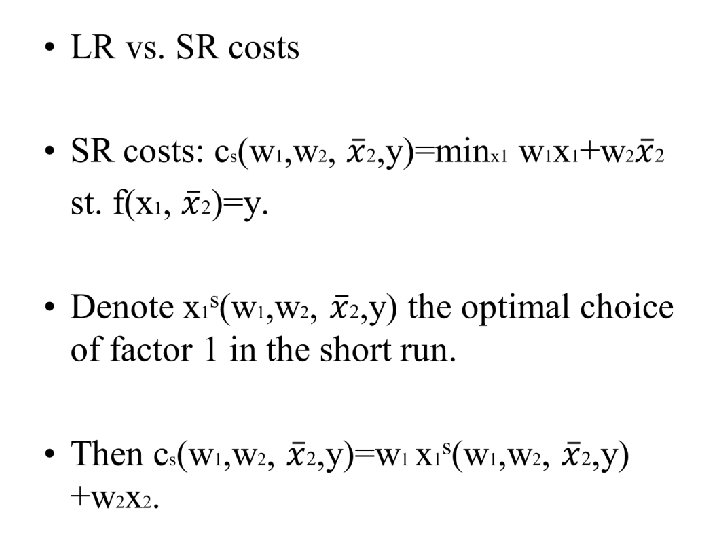
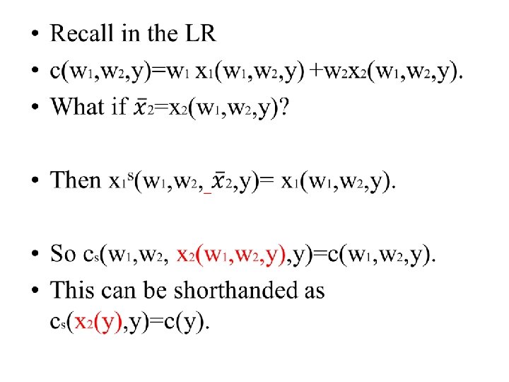
• Intuitively, if in the SR, the fixed factors happen to be at the LR cost minimizing amount, then we don’t have an extra constraint in the SR. • The cost-minimizing amount of the variable inputs in the SR equals that in the LR.

• Normally, cs(x 2, y)≥c(y). • Can we have cs(x 2(y), y)>c(y)? If so, then x 1 s(x 2(y), y)>x 1(y). But notice that in the SR you can also choose x 1(y) to produce y, so this contradicts SR cost minimization. • Hence cs(x 2(y), y)=c(y).

• Sunk costs: expenditures that have been made and cannot be recovered. • They should not affect future decisions. • 100, 000 5 light trucks could sell on the used market for 80, 000, then the sunk cost is 20, 000.

• Chapter 21 Cost Minimization • Key Concept: Cost minimization implies isoquant and isocost are tangent to each other MP 1(x 1*, x 2*)/MP 2(x 1*, x 2*) = w 1/w 2 • LR total cost curve is the lower envelope of the SR total cost curves.